A stochastic multicellular model identifies biological watermarks from disorders in self-organized patterns of phyllotaxis
- Laboratoire de Reproduction de développement des plantes, France
- University of Cambridge, United Kingdom
- The University of Nottingham, United Kingdom
- INRIA Sophia-Antipolis Méditerranée Research Center, France
- AgroParisTech, France
- CIRAD, INRA and INRIA Sophia-Antipolis Méditerranée Research Center, France
Figures
Figure 1
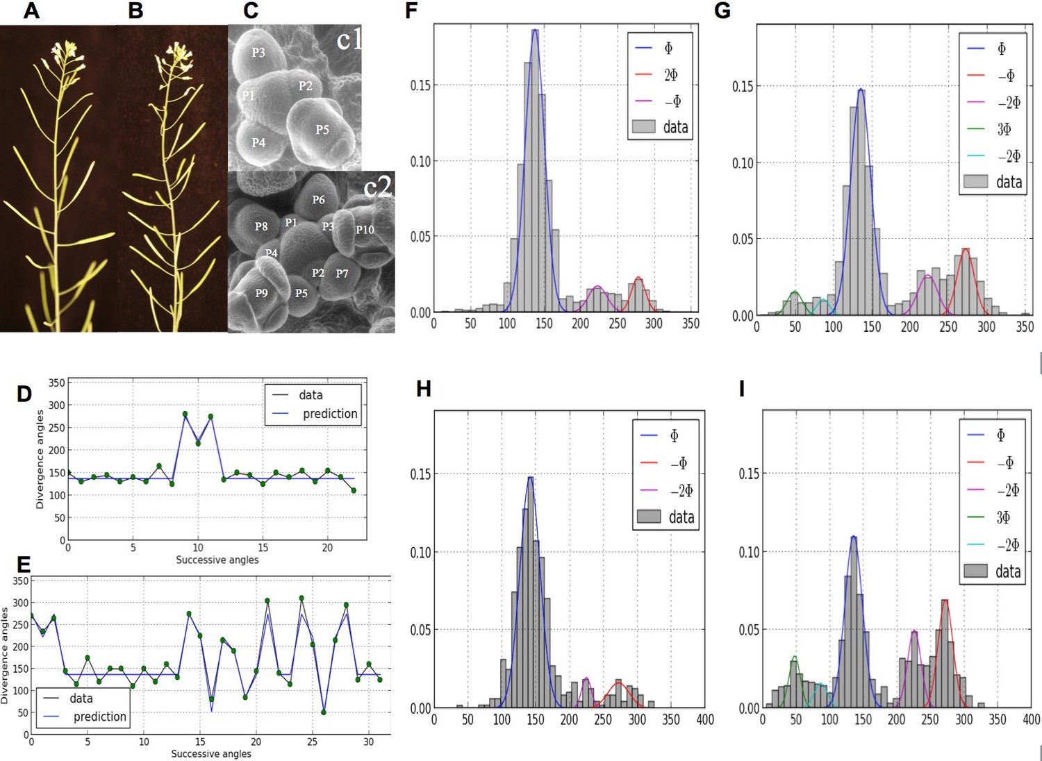
Irregularity in phyllotaxis patterns.
(A) wild type inflorescence of Arabidopsis thaliana showing regular spiral phyllotaxis. (B) aph6 mutant inflorescence showing an irregular phyllotaxis: both the azimuthal angles and the distances between consecutive organs are largely affected. (C1) Organ initiation in the wild type: the size of organs is well hierarchized, initiations spaced by regular time intervals. (C2) Organ initiation in the ahp6 mutant: several organs may have similar sizes, suggesting that they were initiated simultaneously in the meristem (co-initiations). (D) A typical sequence of divergence angles in the WT: the angle is mainly close to (≈137°) with possible exceptions (M-Shaped pattern). (E) In ahp6, a typical sequence embeds more perturbations involving typically permutations of 2 or 3 organs. (F–I) Frequency histogram of divergence angle: wild type (F); ahp6 mutant (G); WS-4, long days (H); WS-4 short days - long days (I).
Figure 2

Permutations can be observed in various species with spiral phyllotaxis.
A schema in the bottom right corner of each image indicates the rank and azimuthal directions of the lateral branches. The first number (in yellow, also displayed on the picture) indicates the approximate azimuthal angle as a multiple of the plant’s divergence angle (most of the times close to 137° or 99°). The second number (in red) corresponds to the rank of the branch on the main stem. (A) Brassica napus (Inflorescence) (B) Muscari comosum (Inflorescence) (C) Alliara petiolata (D) Aesculus hippocastanum (Inflorescence) (E) Hedera Helix (F) Cotinus Dummeri.
Figure 3 with 1 supplement
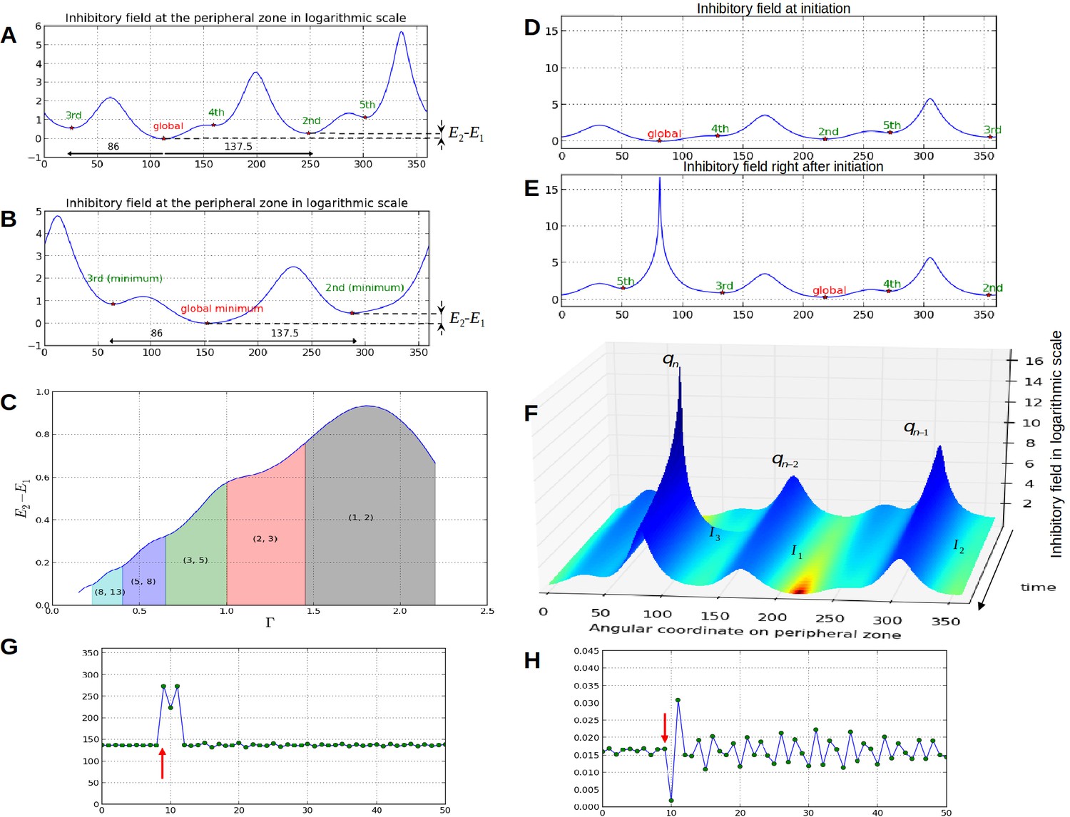
Properties of the inhibition profiles in the classical model and effect of a forced perturbation on divergence angles and plastochrons.
(A) Inhibition variation (logarithmic scale) along the peripheral circle and its global and local minima for a control parameter = 0.975. is the difference in inhibition levels between the kth local minimum and the global minimum. The angular distances between the global minimum and the kth primordiu inhibition m are multiple of the canonical angle (137°). (B) Similar inhibition profile for a control parameter = 0.675 < Γ1. The difference in inhibition levels is higher than in A. (C) Variation of the distance between the global minimum of the inhibition landscape and the local minimum with closest inhibition level (i.e. the second local minimum), as a function of Γ. (D) Inhibition profile just before an initiation at azimuth 80° and (E) just after. (F) Variation of inhibition profile in time. As the inhibition levels of local minima decrease, their angular position does not change significantly, even if new primordia are created (peak qn), color code: dark red for low inhibition and dark blue for high inhibition values. (G) Sequence divergence angles between initiations simulated with the classical model (control parameter ). At some point in time (red arrow), the choice of the next initiation is forced to occur at the 2th local minimum instead of the global minimum. After the forcing, the divergence angle makes a typical M-shaped pattern and returns immediately to the baseline. (H) Corresponding plastochrons: the forcing (red arrow) induces a longer perturbation of the time laps between consecutive organs.
Figure 3—figure supplement 1
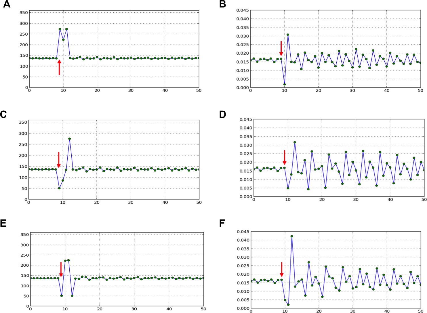
Divergence angle of a series of simulations of the classical model with control parameter =0.975 and for which the choice of the jth local minimum (instead of the global minimum, i.e. j=1) has been forced at a given time-point (red arrow).
After the forcing, the reaction of the classical model is observed. 1. divergence angles (left column) 2. corresponding plastochrons (right column) (A,B) j=2. (C,D) j=3. (E,F) j=3 and j=2 are imposed in this order.
Figure 4
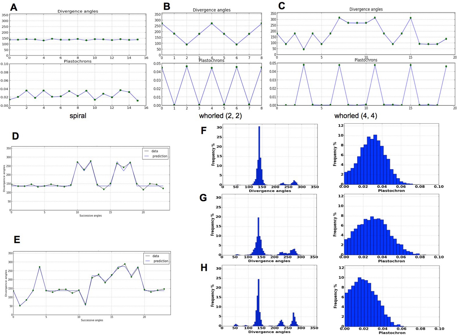
Patterns generated by the stochastic model.
(A) The model generates spiral patterns (in (A–C), up: sequence of simulated divergence angles, down: corresponding plastochrons). (B–C) and whorled patterns. (D) Simple M-shaped permutations simulated by the stochastic model ( = 10.0, = 1.4, = 0.625). (E) More complex simulated permutations involving 2- and 3-permutations ( = 10.0, = 1.4, = 0.9). The permutations are here: [4, 2, 3], [14, 13, 12], [16, 15], [19, 18]. (F) Typical histogram of simulated divergence angles and corresponding plastochron distribution for = 11.0, =1.2, = 0.8. (G) Histogram of simulated divergence angles and corresponding plastochron distribution for = 9.0, = 1.2, = 0.8 (H) Histogram of simulated divergence angles and corresponding plastochron distribution for = 9.0, = 1.2, = 0.625.
Figure 5
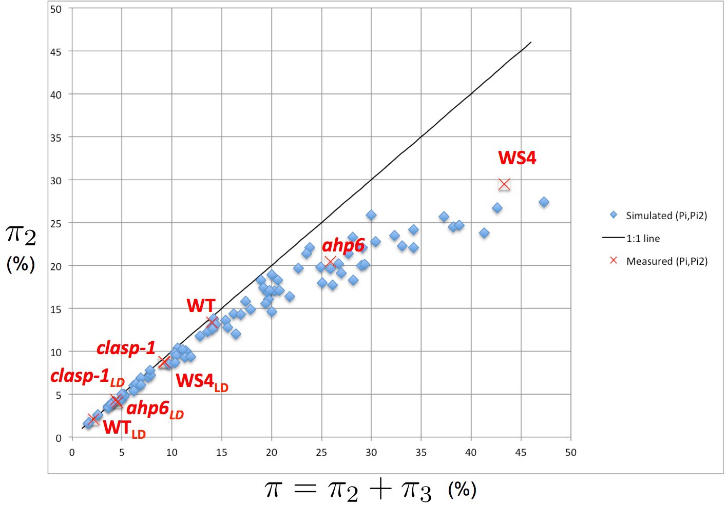
Intensity of 2-permutations as a function of the total amount of perturbations.
As the perturbation intensity increases, the percentage of 2-permutations decreases in a non-linear way to the benefit of more complex 3-permutations. The diagonal line denotes the first bisector. In red: values of 2- and 3-permutations observed in different mutants and ecotypes of Arabidopsis thaliana (Besnard et al., 2014; Landrein et al., 2015 and this study) placed on the plot of values predicted by the stochastic model.
-
Figure 5—source data 1
Source files for simulated permutation intensities.
This file contains a table showing the variation of permutation intensities with model parameters. We ran simulations using the SMPmacro-max model for different parameter values where the local minima of inhibition profile indicate the potential initiation sites (for this, the inhibitory field values were estimated at 360 sampling points regularly distributed around the periphery of the central zone). We then used the combinatorial model (Refahi et al., 2011) to detect permutations in the simulated sequences. The model has mainly three parameters, , and . For each parameter value of , and , we run sixty simulations. Each simulation generated a sequence of 25 divergence angles. We then analyzed the sequences using the combinatorial model to detect permutation patterns.
- https://doi.org/10.7554/eLife.14093.012
Figure 6 with 1 supplement
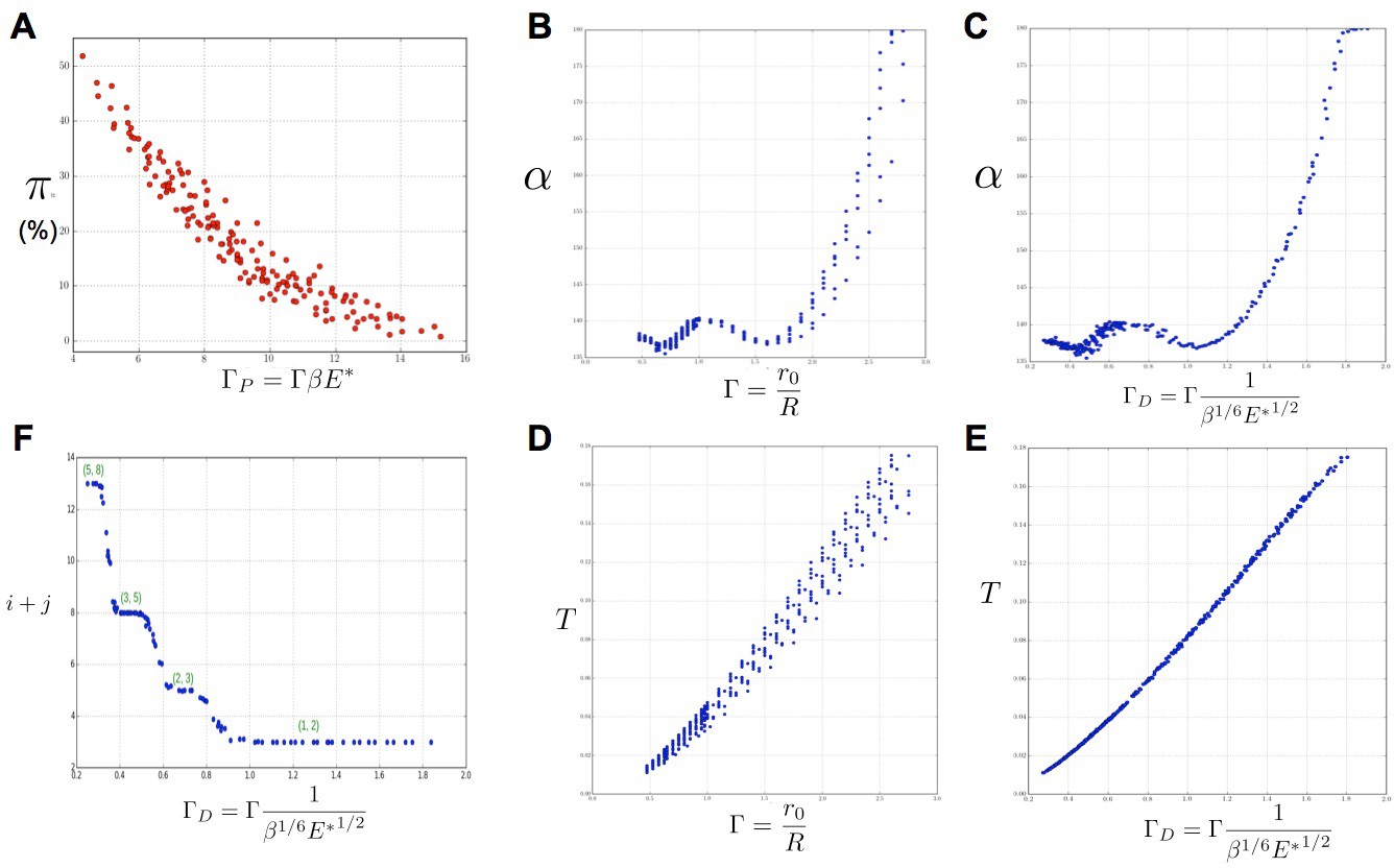
Key parameters controlling phyllotaxis phenotypes in the stochastic model.
Phyllotaxis sequences were simulated for a range of values of each parameter , , . Each point in the graph corresponds to a particular triplet of parameter values and represents the average value over 60 simulated sequences for this triplet. (A) Global amount of perturbation as a function of the new control parameter . (B) Divergence angle as a function of the control parameter of the classical model on the Fibonacci branch. (C) Divergence angle as a function of the new control parameter on the Fibonacci branch (here, we assume s = 3, see Appendix 1—figure 6 for more details). (D) Plastochron as a function of control parameter of the classical model . (E) Plastochron as a function of the new control parameter . (F) Parastichy modes identified in simulated sequences as a function of . Modes are represented by a point . The main modes (1,2), (2,3) … correspond to well marked steps. (Figure 5—source data 1)
Figure 6—figure supplement 1
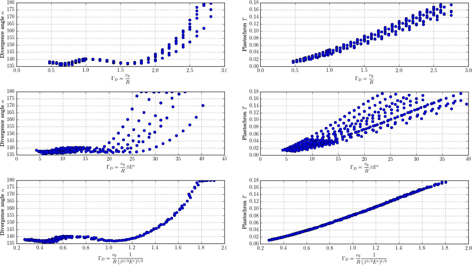
New control parameter for divergence angle and plastochrons.
Each graph is made up of points that correspond to different values of the parameters of the stochastic model. Left column: different trials to define a control parameter for divergence angles . Right column: different tries to define a control parameter for the plastochrons. For the parameter , both clouds of points collapse on a single curve (we assume here that s = 3, see Appendix 1—figure 6 for more details).
Figure 7
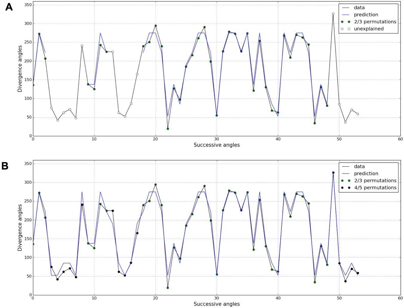
Detection of higher-order permutations in WS4.
The detection algorithm (see ref [7] for details) searches plausible angle values, i.e. values within the 99% percentile given the Gaussian like distributions fitted in Figure 1, such that the overall sequence is n-admissible, i.e. composed of permuted blocks of length at most n. (A) When only 2- and 3-permutations are allowed, some angles in the sequences cannot be explained by (i.e. are not plausible assuming) permutations (the blue line of successfully interpreted angles is interrupted). (B) Allowing higher order permutations allows to interpret all the observe angles as stemming from 2-, 3- 4- and 5-permutations (the blue line covers the whole signal). Organs indexes involved in permutations: [3, 2], [5, 8, 6, 4, 7], [13, 12], [16, 14, 17, 15], [19, 18], [22, 21], [24, 25, 23], [27, 26], [30, 29], [32, 31], [35, 34], [39, 40, 38], [43, 42], [46, 45], [48, 49, 47], [52, 50, 53, 51].
Figure 8
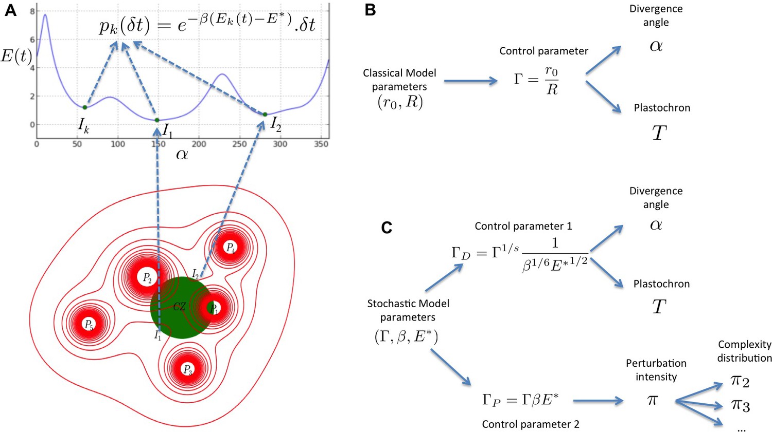
Structure of the stochastic model.
(A) Inhibitory fields (red), possibly resulting from a combination of molecular processes, are generated by primordia. On the peripheral region of the central zone (CZ, green), they exert an inhibition intensity that depends on the azimuthal angle (blue curve). At any time t, and at each intensity minimum of this curve, a primordium can be initiated during a time laps with a probability that depends on the level of the inhibition intensity at this position. (B) Relationship between the classical model parameters and its observable variables. A single parameter controls both the divergence angle and the plastochron. (C) Relationship between the stochastic model parameters and its observable variables. The stochastic model of phyllotaxis is defined by 3 parameters ,, . The observable variables , and … are controlled by two distinct combinations of these parameters: controls the divergence angle and plastochron while controls the global percentage of permutated organs , which in turns controls the distribution of permutation complexities: ….
Appendix 1—figure 1
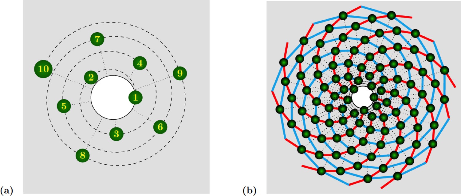
Spiral phyllotaxis with divergence angle and different distributions of radial positions.
(a) The first 10 primordia are depicted, with the generative spiral as a dashed line. The angle between successive organs is always equal to . The nearest neighbours of primordium are and , hence the mode of this pattern is . (b) 100 primordia are depicted, along with the 8 (resp. 13) parastichies oriented anticlockwise (resp. clockwise) indicated in cyan (resp. red), hence the mode of this pattern si .
Appendix 1—figure 2
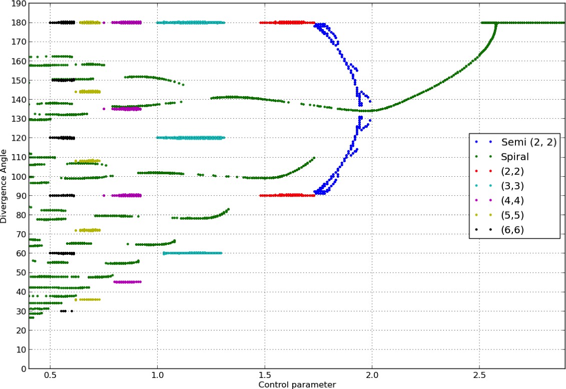
Bifurcation diagram in the Snow and Snow model.
We used a sample of the interval with steps of or less (refinements were performed in areas with higher numbers of branches). For each value of , we ran simulations of the classical model with (i) spiral initial conditions for divergence angles taking integer values in , and plastochrons taking values in a sample of 128 points between and , (ii) whorled initial conditions for the same samples of divergence angles and plastochrons and all jugacies . For each simulation, we estimated the final divergence angle and phyllotactic mode, and reported these in the graph above (abscissa: , ordinate: , color code: mode).
Appendix 1—figure 3
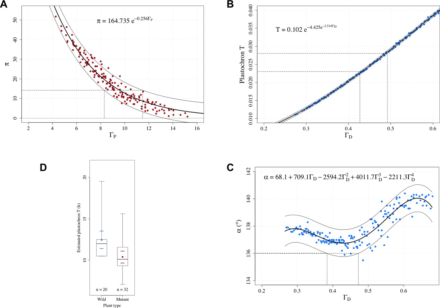
Estimation of control parameters from observable phyllotaxis variables.
(A) An exponential model was fitted to the simulated data of and using the Gauss-Newton least squares method (Bates and Watts, 2007); for the fitted model, an approximate 95% prediction band was then computed by assuming the random error terms additive and i.i.d. normally distributed. The range of possible values [8.30, 11.49] that could yield the observed value 14.2 was determined by the prediction band. (B) A Gompertz function was fitted to the simulated data of plastochron and using the Gauss-Newton least squares method (Bates and Watts, 2007); for the fitted model, an approximate 95% prediction band was then computed by assuming the random error terms additive and i.i.d. normally distributed. The range of possible values [0.427, 0.492] that could yield the observed range of plastochron values [0.023, 0.028] was determined by the prediction band. (C) A 4th degree polynomial was fitted to the simulated data of angle and using the least squares method; for the fitted model, an approximate 95% prediction band was then computed by assuming the random error terms additive and i.i.d. normally distributed. The range of possible values [0.384, 0.472] that could yield the observed angle value of 136° was determined by the prediction band. (D) Distributions of the estimated plastochrons in the groups of wild-type and mutated Arabidopsis plants in the experiments of Besnard et al., 2014. The box depicts the inter-quartile range bisected by the median, and the whiskers reach out to the extreme values in the group; the colored point denotes the arithmetic mean, and the colored dashes indicate twice the standard error of the mean; stands for the number of plants in the group.
Appendix 1—figure 4
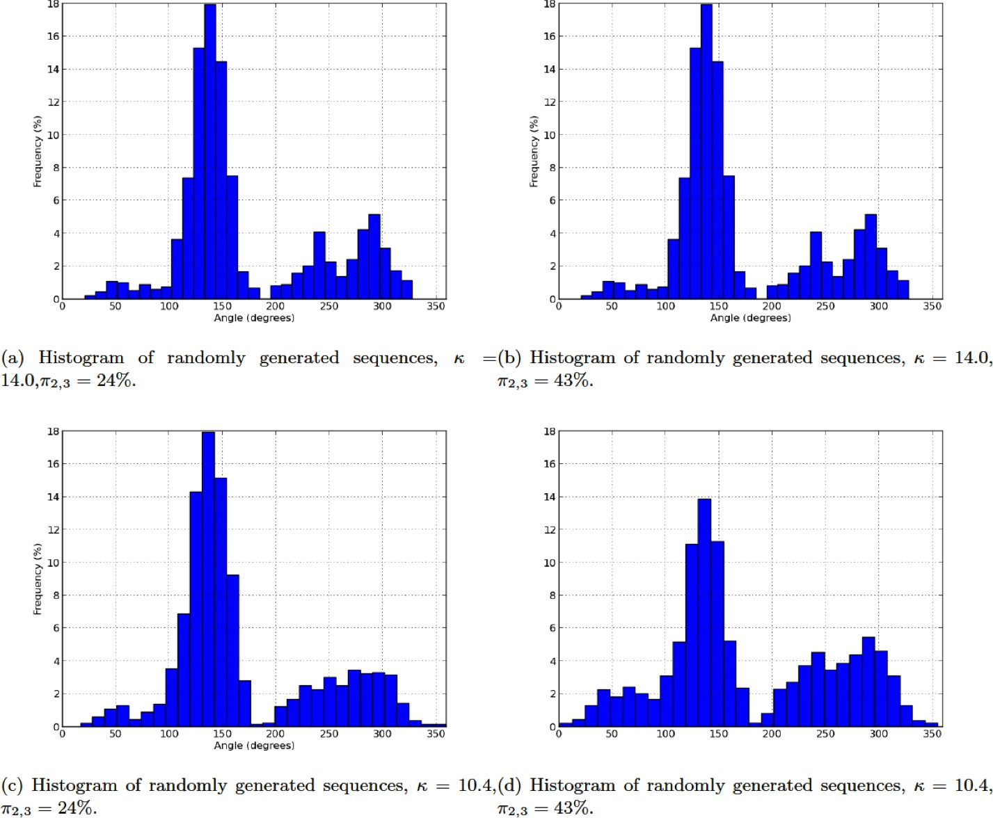
Histogram of randomly generated sequences.
(a) Histogram of randomly generated sequences, ,. (b) Histogram of randomly generated sequences, , . (c) Histogram of randomly generated sequences, , . (d) Histogram of randomly generated sequences, , .
Appendix 1—figure 5

Role of the control parameters for the based inhibition function.
(a–b) Average plastochron ratio as a function of and , respectively. (c) Number of permutations as a function of .
Appendix 1—figure 6
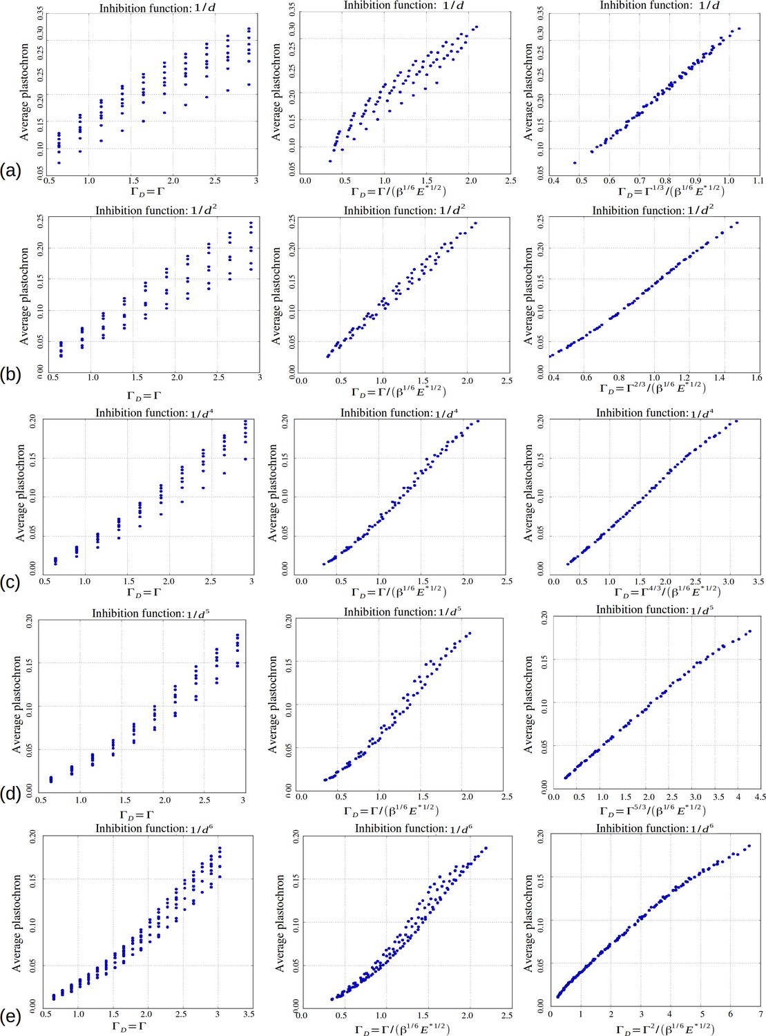
Role of the control parameters for the power law inhibition function, with rows (a–e) corresponding respectively to a steepness .
First two columns: average plastochron ratio as a function of and , respectively. Third column: average plastochron ratio as a function of .
Appendix 1—figure 7
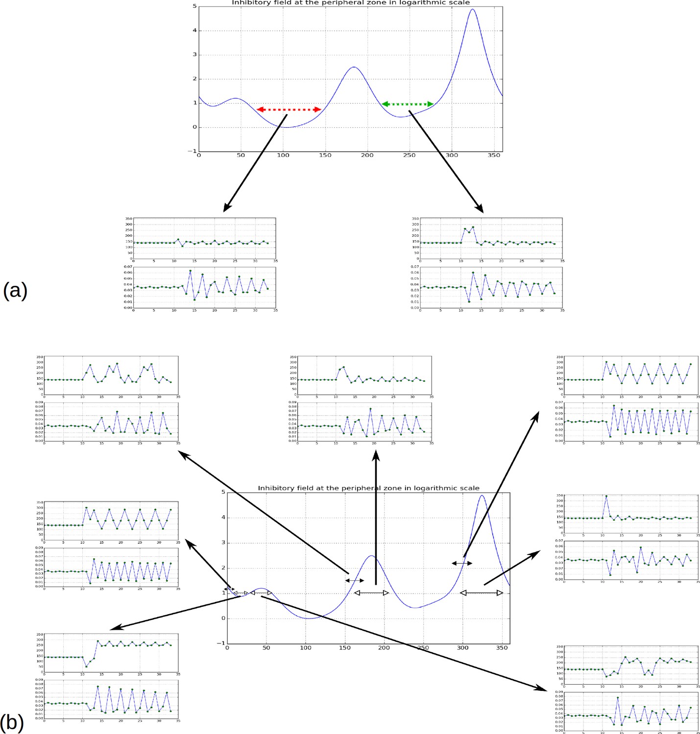
Effect of forcing initiation in different regions of the inhibitory field profile.
(a) As reported in Figure 2H, forcing a primordium near the first or second local minima does not affect the phyllotactic mode permanently, but simply forces a 2-permutation in the case of the second minimum. (b) When primordia are introduced near the highest or second highest local maxima, the system returns to its previous pattern. Near the third maximum or the third minimum, the system changes pattern, in the shown simulation it converges to a spiral oriented in the opposite direction to the previous spiral (i.e. instead of ); a 2-permutation can be seen in the new spiral for the third maximum. New primordia introduced far from any maximum or minimum (black headed arrows) tend to disrupt the phyllotactic mode more significantly, converging to whorled patterns (primordia forced near 0 or near 290), or patterns involving high numbers of successive permutations (primordium forced near 150).
Videos
Video 1
Temporal variation of the inhibitory profile around the central zone in the classical model for a large value of the parameter .
The number of inhibition mimima is stable (3) in time. When the absolute minimum reaches the initiation threshold (here E = 0), a primordium is created that instantaneously creates a strong inhibition locally, which suddenly increases the inhibition level at its location. Between initiations, local minima regularly decrease in intensity due to the fact that growth is moving existing primordia away from the center. This movement is accompanied by a slight drift in position common to all primordia (here to the right).
Video 2
Temporal variation of the inhibitory profile around the central zone in the classical model for a small value of the parameter .
The dynamics is similar to that of small except that the number of local minima of inhibition is higher (here 5) and that the distance between two consecutive minima is lower.
Video 3
Temporal variation of the inhibitory profile around the central zone in the stochastic model for a small value of the parameter .
Here, due to stochasticity, global minimum is not always the one that triggers an initiation. The dynamics of the divergence angle and of the plastochron are shown in the bottom graphs to interpret the model's initiations based on the inhibition levels.
Appendix 2—video 1
Dynamics of the divergence angles as well as the inhibitory field at the peripheral zone.
The stochastic model generates a Fibonacci spiral including two 2-permutations from a random initial inhibitory field. For more precise information about the initial condition see Supplementary information.
Appendix 2—video 2
Dynamics of the divergence angles as well as the inhibitory field at the peripheral zone.
The stochastic model generates a Fibonacci spiral from a random initial inhibitory field. It takes some time to converge to 137 degrees. For more precise information about the initial condition see Supplementary information.
Appendix 2—video 3
Dynamics of the divergence angles as well as the inhibitory field at the peripheral zone.
The stochastic model generates a Fibonacci spiral pattern including a 2-permutation pattern at the beginning before converging to 137 degrees. For more precise information about the initial condition see Supplementary information.
Appendix 2—video 4
Dynamics of the divergence angles as well as the inhibitory field at the peripheral zone.
The stochastic model generates a 2-whorled pattern from no pre-existing organs. For more precise information about the initial condition see Supplementary information.
Appendix 2—video 5
Dynamics of the divergence angles as well as the inhibitory field at the peripheral zone.
The stochastic model generates a 2-whorled pattern from a random initial inhibitory field. For more precise information about the initial condition see Supplementary information.
Appendix 2—video 6
Dynamics of the divergence angles as well as the inhibitory field at the peripheral zone.
The stochastic model generates a 2-whorled pattern from a random initial inhibitory field (second run). For more precise information about the initial condition see Supplementary information.
Appendix 2—video 7
Dynamics of the divergence angles as well as the inhibitory field at the peripheral zone.
The stochastic model generates a 2-whorled pattern from no pre-existing organs (second run). For more precise information about the initial condition see Supplementary information.
Appendix 2—video 8
Dynamics of the divergence angles as well as the inhibitory field at the peripheral zone.
The stochastic model generates a 4-whorled pattern from no pre-existing organs. For more precise information about the initial condition see Supplementary information.
Appendix 2—video 9
Dynamics of the divergence angles as well as the inhibitory field at the peripheral zone.
The stochastic model generates a 4-whorled pattern from a random initial inhibitory field. For more precise information about the initial condition see Supplementary information.
Appendix 2—video 10
Dynamics of the divergence angles as well as the inhibitory field at the peripheral zone.
The stochastic model generates a 4-whorled pattern from a random initial inhibitory field (second run). For more precise information about the initial condition see Supplementary information.
Appendix 2—video 11
Dynamics of the divergence angles as well as the inhibitory field at the peripheral zone.
The stochastic model generates a 4-whorled pattern from no pre-existing organs (second run). For more precise information about the initial condition see Supplementary information.
Appendix 2—video 12
Dynamics of the divergence angles as well as the inhibitory field at the peripheral zone showing multiple initiation sites.
The SMPmicro variant was used instead of SMPmacro-max used in the previous simulations. With SMPmicro, a primodium may be initiated at any cell independently of the others. This makes it possible to two primordia initiation in the same valley. A single initiation site is marked in green and multiple simultaneous initiation sites are marked in red. An initial spiral pattern of 150 preexisting primordia has been used as initial condition.
Appendix 2—video 13
Same video as Appendix 2—video 12 with lower fps.
https://doi.org/10.7554/eLife.14093.046Tables
Appendix 1-table 1
Observed phyllotaxic variables on plants grown in short day and then in long day conditions. % permuted organs is shown as a number followed by 2 other numbers in parentheses, i.e.
| Short day - Long day | Col0 | WS4 | clasp-1 | ahp6 |
| #angles/#sequences | 704/29 | 1046/25 | 619/17 | 2815/89 |
| Estimated # 2-permutations | 49 | 154 | 28 | 297 |
| Estimated # 3-permutations | 2 | 52 | 1 | 53 |
| % unexplained angles | %2.7 | %7.7 | %1.1 | %2 |
| Estimated % permuted organs | 14(13.37,0.82) | 43.3(29.45,14.91) | 9.2(8.81, 0.47) | 25.9(20.45,5.47) |
| Estimated average | 136.4 | 136 | 138.0 | - |
| Estimated standard deviation | 5.5 | 2.3 | 6 | - |
| # Lucas sequences | 0 | 0 | 0 | 0 |
| Average measured plastochron (h) | 7.5 | 5.1 | 19 | 10.6 |
| Plastochron ratio | 1.12 | 1.08 | 1.135 | - |
| Estimated plastochron (equ. 12) | 0.0227 | 0.0154 | 0.0253 | - |
| Estimated | 0.430 | 0.325 | 0.450 | - |
| Estimated (in ) | [8.7,11.4] | [5.2,5.8] | [9.6,12.3] | [6.7,8.7] |
Appendix 1–table 2
Observed phyllotaxic variables on plants grown in long day conditions only. % permuted organs is shown as a number followed by 2 other numbers in parentheses, i.e. .
| Long day only | Col0 | WS4 | clasp-1 | ahp6 |
| #angles/#sequences | 1193/34 | 487/15 | 667/19 | 965/27 |
| Estimated # 2-permutations | 13 | 22 | 14 | 22 |
| Estimated # 3-permutations | 0 | 1 | 1 | 0 |
| % unexplained angles | %2.6 | %3.6 | %4.3 | %0.1 |
| Estimated % permuted organs | 2.12(2.12,0) | 9.3(8.76, 0.6) | 4.52(4.08, 0.44) | 4.4(4.44,0) |
| Estimated average | 136.4 | 141.4 | 128.1 | - |
| Estimated standard deviation | 10.7 | 6.8 | 20.46 | - |
| # Lucas sequences | 0 | 0 | 6 | 0 |
| Average plastochron (h) | 10 | 6.3 | 21 | 9.5 |
| Plastochron ratio | 1.15 | 1.115 | 1.145 | - |
| Estimated plastochron (equ. 12) | 0.0280 | 0.0218 | 0.0271 | - |
| Estimated | 0.485 | 0.410 | 0.475 | - |
| Estimated (in ) | [12.8,15.1] | [10.0,12.0] | [11.7,14.2] | [11.8,14.3] |
Appendix 1–table 3
Combinatorial models permutation detection precision on randomly generated noisy data.
| \ | 24% | 43% |
| 14 | 100% | 98.5% |
| 10.4 | 99% | 98% |
Appendix 1–table 4
1 degree (in the paper), permutation rates and average divergence angle.
| \ | 10 | 12 |
|---|---|---|
| 0.65, 1 | 30.0 (22.3, 7.7), 136 | 18.4(15.7, 2.8), 136.8 |
| 0.75, 1 | 30.7(21.2, 9.5), 136.2 | 15.5 (11.5, 0.9), 137.3 |
| 0.85, 1 | 17.6(13.5, 4.1), 138.5 | 15.5(11.9, 3.5), 137.3 |
| 0.95, 1 | 11.7(9.5, 1.8), 139.9 | 4.8(4.4, 0.4)140.1 |
Appendix 1–table 5
2 degrees, permutation rates and average divergence angle.
| \ | 10 | 12 |
|---|---|---|
| 0.65 , 1 | 31.8(24.3,7.4), 136.4 | 19.7(18.2,1.5), 136.6 |
| 0.75, 1 | 27.1(16.9,10.2), 136 | 11.8(10.2,1.6), 136.5 |
| 0.85, 1 | 19.8(14.7,5.2), 137.3 | 11.0(9.9,1.1), 137.7 |
| 0.95, 1 | 13.6(12.6,1.0), 138.7 | 5.3(5.0,0.3), 139.5 |
Appendix 1–table 6
5 degrees, permutation rates and average divergence angle.
| \ | 10 | 12 |
|---|---|---|
| 0.65, 1 | 32.9(25.1,7.8), 136.1 | 21.3(17.5,3.8), 136.1 |
| 0.75, 1 | 35.2(23.3,11.9), 135.7 | 18.1(16.0,2.1), 136.3 |
| 0.85, 1 | 16.6(12.9,3.7), 137.9 | 8.9(7.5,1.4), 137.9 |
| 0.95, 1 | 10.0(8.2,1.9), 139.4 | 4.3(4.3,0.0), 139.9 |
Appendix 1–table 7
10 degrees, permutation rates and average divergence angle.
| \ | 10 | 12 |
|---|---|---|
| 0.65, 1 | 36.7(24.7,12.0), 136.5 | 29.7(22.0,7.6), 136.2 |
| 0.75, 1 | 29.0(22.4,6.6), 136.9 | 25.3(20.8,4.5), 136.7 |
| 0.85, 1 | 24.2(17.4,6.8), 135.9 | 21.0(17.5,3.5), 134.8 |
| 0.95, 1 | 13.2(13.2,0.0), 139.3 | 9.4(8.8,0.6), 139.5 |
Appendix 1–table 8
Permutation rates for the based inhibition rate, with ; permutation rates and average divergence angle.
| \ | 7 | 8 | 10 | 12 |
|---|---|---|---|---|
| 0.45, 1 | 35.9(25.9,10.0), 138.5 | 25.1(20.9,4.2), 138.3 | ||
| 0.45, 1.2 | 45.9(25.6,20.3), 138.8 | 42.4(30.1,12.3), 138.5 | 26.8(21.1,5.7), 138.1 | 17.7(16.0,1.6), 137.9 |
| 0.55, 1 | 44.3(27.4,16.8), 138.0 | 36.1(26.5,9.6), 138.2 | 23.3(20.1,3.1), 137.5 | 15.9(14.5,1.3), 137.4 |
| 0.55, 1.2 | 36.7(25.8,10.9), 138.0 | 28.0(20.4,7.6), 137.9 | 17.1(15.5,1.6), 137.7 | 13.9(13.9,0.0), 137.5 |
| 0.65, 1 | 39.0(26.3,12.8), 135.7 | 30.4(23.7,6.7), 136.3 | 15.3(14.1,1.1), 136.3 | 10.3(9.7,0.6), 136.8 |
| 0.65, 1.2 | 27.7(22.2,5.6), 136.4 | 19.9(17.1,2.8), 136.7 | 10.6(10.2,0.4), 136.7 | 4.3(4.3,0.0), 136.7 |
| 0.75, 1 | 40.2(23.0,17.2), 135.2 | 32.2(20.9,11.3), 135.1 | 17.6(14.4,3.2), 135.8 | 10.9(10.3,0.5), 136.3 |
| 0.75, 1.2 | 31.1(22.6,8.5), 135.0 | 21.3(18.1,3.2), 136.0 | 11.1(10.0,1.1), 136.5 | 6.7(6.2,0.5), 137.1 |
| 0.85, 1 | 27.4(17.5,9.9), 137.6 | 19.2(14.4,4.8), 137.2 | 5.9(5.9,0.0), 138.0 | 4.4(4.2,0.2), 138.1 |
| 0.85, 1.2 | 21.5(15.8,5.8), 136.4 | 14.4(13.0,1.4), 136.9 | 5.6(5.6,0.0), 137.6 | 3.1(3.0,0.1), 138.0 |
| 0.95, 1 | 21.0(16.2,4.9), 138.9 | 14.8(10.7,4.0), 138.6 | 3.7(3.7,0.0), 139.6 | |
| 0.95, 1.2 | 15.4(12.4,3.1), 138.4 | 8.5(7.3,1.2), 138.9 | 2.9(2.9,0.0), 139.4 | |
| 1.05, 1 | 22.4(16.8,5.6), 139.6 | 13.1(11.0,2.1), 139.2 | 2.4(2.4,0.0), 139.6 | |
| 1.05, 1.2 | 10.2(9.3,0.9), 139.5 | 5.8(5.7,0.1), 139.7 | 2.1(2.1,0.0), 139.9 |
Appendix 1–table 9
Growth rate changed, .
| \ | 10 | 12 |
|---|---|---|
| 0.65, 1 | 29.0(21.0,8.0), 136.2 | 17.7(16.2,1.5), 136.6 |
| 0.75, 1 | 27.4(19.8,7.6), 135.4 | 15.8(14.6,1.2), 136.2 |
| 0.85, 1 | 14.7(11.3,3.4), 137.7 | 10.5(9.8,0.6), 138.0 |
| 0.95, 1 | 8.0(6.9,1.1), 139.3 | 4.3(4.1,0.2), 139.3 |
Appendix 1–table 10
Noise added to the peripheral zone.
| \ | 10 | 12 |
|---|---|---|
| 0.75, 1 | 29.2(19.5,9.7), 135.9 | 16.8(14.2,2.6), 136.7 |
| 0.75, 1.2 | 17.2(14.8,2.3), 136.4 | 14.6(12.5,2.1), 136.1 |
| 0.85, 1 | 23.6(16.0,7.7), 136.6 | 12.3(11.2,1.1), 137.7 |
| 0.85, 1.2 | 16.5(14.2,2.2), 135.7 | 9.2(8.3,0.9), 137.2 |
| 0.95, 1 | 12.5(11.4,1.1), 139.4 | 6.9(6.7,0.2), 139.4 |
| 0.95, 1.2 | 8.6(7.5,1.1), 138.9 | 2.4(2.4,0.0), 138.6 |
Download links
A two-part list of links to download the article, or parts of the article, in various formats.
Downloads (link to download the article as PDF)
Open citations (links to open the citations from this article in various online reference manager services)
Cite this article (links to download the citations from this article in formats compatible with various reference manager tools)
A stochastic multicellular model identifies biological watermarks from disorders in self-organized patterns of phyllotaxis
eLife 5:e14093.
https://doi.org/10.7554/eLife.14093


