Mapping cortical mesoscopic networks of single spiking cortical or sub-cortical neurons
- Kinsmen Laboratory of Neurological Research, Canada
- Beijing Institute for Brain Disorders, Capital Medical University, China
- Djavad Mowafaghian Centre for Brain Health, University of British Columbia, Canada
- University of British Columbia, Canada
Figures
Figure 1 with 2 supplements
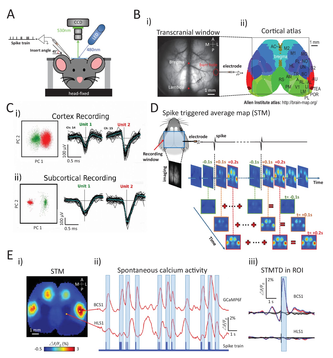
Experimental setup and multichannel electrode recordings and spike classification.
(A) Set-up for simultaneous wide-field calcium imaging and single unit recording using a glass pipette or laminar silicon probe. (Bi) Top view of wide-field transcranial window and (ii) cortical atlas adapted from the Allen Institute Brain Atlas. (C) Example of (i) cortical and (ii) subcortical pairs or spike recordings from separate channels showing the isolation in the two principal components axes. (D) The generation of a spike-triggered average map (STM) for unit located in barrel cortex. (Ei) STM generated from single neuron with 1158 spikes recorded in right barrel cortex. (ii) Red traces: Spontaneous calcium activity recorded from two different cortical areas (BCS1 and HLS1). Blue trace: spontaneous spiking activity recorded simultaneously from right BCS1. (iii) STMTD generated from average of calcium activity time-locked with each spike (red) and random spike (see Materials and methods, black, blue: subtraction of spike and random spike-evoked responses) in region-of-interest (ROI). These examples results were from mice under anesthesia. Source files for the generation of spike-triggered average map (STM) can be found at http://goo.gl/nHF29I. The folder ‘Matlab code and source data’ (see the sublink of https://github.com/catubc/sta_maps) contains calcium images (‘tif’ file), spike train and Matlab code used for the generation of STM shown in Figure 1E. The ‘tif’ file cannot not be viewed with a standard picture viewer, but must be viewed with a program, such as ‘ImageJ’. Spike times were exported as ‘txt’ file. Matlab code (named ‘STA_eLife.m’) was used for reading images and spike time files and generating STM.
Figure 1—figure supplement 1

Spectral distribution of the spontaneous activity.
Average Fourier Transform (±SEM) of the resting state activity of green GCaMP6 fluorescence (black curve, n = 20) and green 532 nm reflectance (gray curve, n = 11) within barrel cortex of awake Ai93 mice.
Figure 1—figure supplement 2
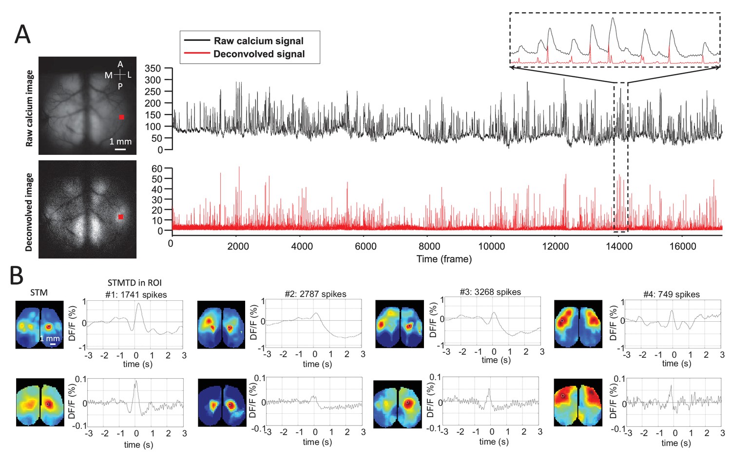
Deconvolution analysis of GCaMP data.
(A) Top: raw calcium image and time course of calcium dynamics in region of interest (ROI). Bottom: deconvolved calcium image and time course of deconvolved calcium dynamics ROI. (B) Top: spike-triggered average map (STM) and STM temporal dynamic (STMTD) of raw data in ROI. Bottom: STM and STMTD of deconvolved data in ROI for spikes from the same neurons. These neurons were recorded in thalamus under anesthesia.
Figure 2
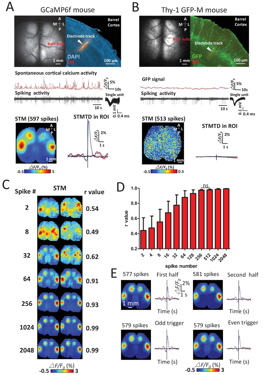
Sensitivity and specificity of STMs.
(A) Simultaneous calcium and spiking activity recording in GCaMP6f mouse and STM yielded from single unit recorded in barrel cortex. (B) Simultaneous GFP fluorescence and spiking activity recording in Thy-1 GFP-M mouse and STM yielded from single unit recorded in barrel cortex resulted in no clear regional map. (C) STMs generated from a subset of spikes (2–2048, on the left) randomly chosen in one experiment. Correlation coefficients (r-value on the right) between STMs were used to evaluate the consistency of mapping. In this example, STMs generated by more than 64 spikes generated a correlation >0.9 and revealed high similarity between the pairs of SPMs made using the same number of spikes. (D) Distribution of correlation values between pairs of STM for an increasing number of spikes. No significant change in r-value distribution was observed for 512 spikes in comparison to 256 spikes (Mann Whitney test, p=0.126, U = 948.5, 256 spikes group n = 58, r-value = 0.97 ± 0.01, mean ± SD; 512 spikes group n = 40, r-value = 0.98 ± 0.01). (E) STMs and profile of responses computed using spikes divided into halves or even-odd sets. These examples were performed under anesthesia.
Figure 3 with 2 supplements
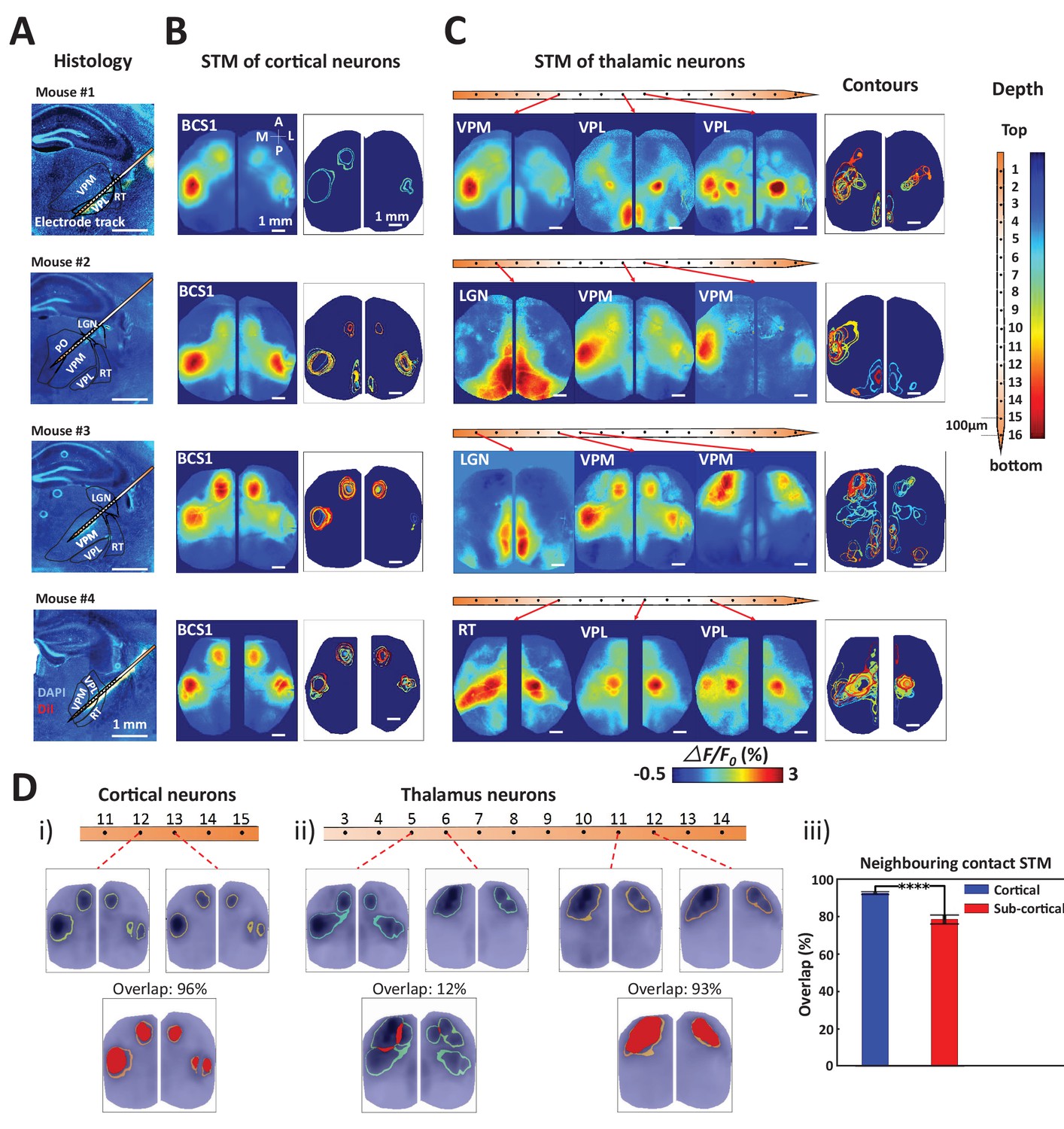
Topographic properties of cortical and thalamic STM.
(A) Electrode track for each recording (Blue channel: DAPI, yellow: DiI). (B) STM and overlay contours of neurons recorded in barrel cortex in the same animal. Each color represents one STM contour. (C) STM and overlay contours of neurons recorded in thalamus in the electrode track presented in panels A and B. Color bar in the right side indicated the depth of each recording site. (D) Diversity of overlap of STMs between neurons on neighboring laminar electrode channels. (i) Example of overlapping STMs (red area) between two cortical neurons recorded on adjacent channels. (ii) Example of overlapping STMs for neighboring pairs of neurons recorded subcortically showing differences across depth. (iii) Average neighboring cortical neuron map overlap (blue: 93%) and neighboring sub-cortical neuron overlap (78%) show significant differences (Mann Whitney test, p<0.0001, U = 617408.0, mean percentage overlap of cortical STM pairs = 92.77% ± 0.23%, mean ± SEM, n = 966; mean percentage overlap of sub-cortical STM pairs = 78.11% ± 0.61%, mean ± SEM, n = 1936). These results are from awake mice (except Mouse #1).
Figure 3—figure supplement 1
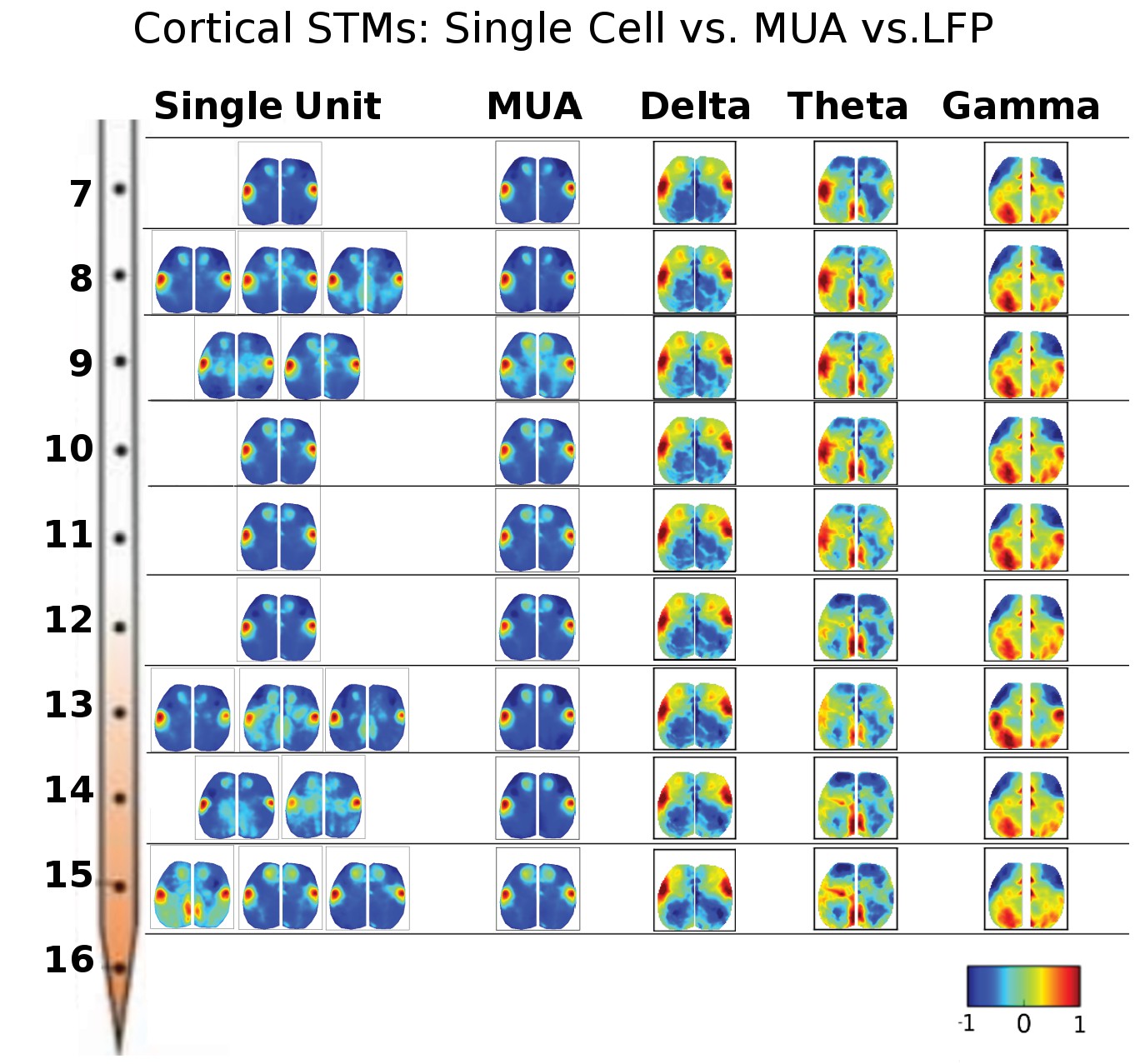
STMs were computed at different depths of the electrode using single cell spikes, Multi-Unit-Activity (MUA) and local field potential (LFP) amplitude.
Single unit STMs were computed (see Materials and methods) for up to three representative cells at each depth. MUA STMs at each electrode were computed using all spiking activity over a threshold (>4 times the standard deviation of the high-pass record divided by 0.675). LFP-triggered STMs were computed by convolving the average LFP amplitude in each imaging time frame with the frame before averaging. Thus, imaging frames where the average LFP amplitude was large and positive contributed substantially to the STM, while frames where the average LFP values were low did not. The various band-passed LFP values used were delta: 0.1–4 Hz, theta: 4–8 Hz and gamma: 25–100 Hz. Single cell STMs at each depth – and across depth – have similar motifs to each other and MUA-triggered STMs. LFP-triggered STMs are substantially different from single cell and MUA-triggered STMs and across different LFP frequency bands (see main text).
Figure 3—figure supplement 2
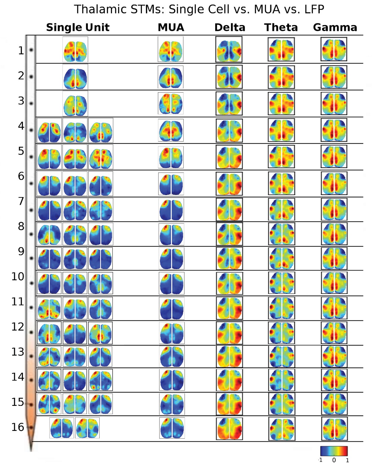
Thalamic STMs: Spike vs LFP.
STMs were computed at different depths of the electrode using single cell spikes, Multi-Unit-Activity (MUA) and LFP amplitude (See Figure 3—figure supplement 1). In contrast to cortical STMs, single thalamic neurons at some depths have more varied motifs (e.g. electrodes 4, 11, 12, 15), while MUA-triggered STMs appear similar across large thalamic regions (e.g. electrodes: 4–16). LFP-triggered STMs are different from single cell and MUA-triggered STMs and across different LFP frequency bands (see main text). LFP, local field potential.
Figure 4
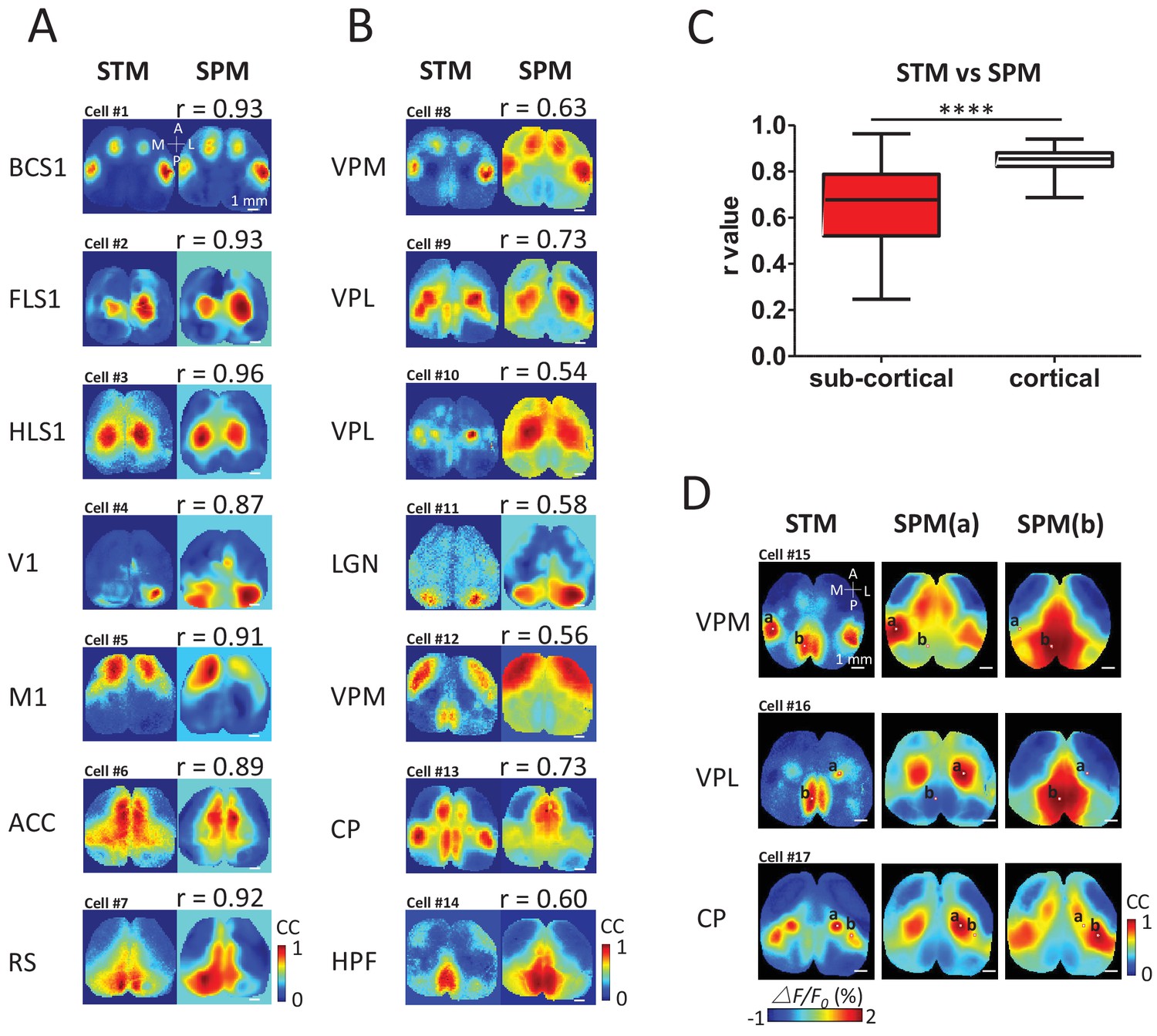
STM compared with seed pixel correlation maps (SPM).
(A) Cortical STM (left) and the best fitting SPM (right) according to correlation coefficient (cc) values for different electrode placements (text to the left of panel). Similarity was calculated by measuring the r-value Pearson coefficient between each pair of map pixels (in title). Group data from 12 GCaMP6f mice are reported in panel C. (B) Sub-cortical STM (left) and the most similar SPM (right). Cells #2 and #4 were from GCaMP6s mice. Cells #3, 5–7, 11 were from GCaMP3 mice. Other cells were from GCaMP6f mice. These examples were performed under anesthesia. (C) Distribution of r-values (Mann Whitney test, p<0.0001, U = 5227, sub-cortical group n = 246 r-value=0.64 ± 0.18, mean SD; cortical group n = 168 r-value=0.85 ± 0.04, mean ± SD). (D) Examples of sub-cortical STMs compared with pairs of SPMs for seed indicated by ‘a’ and ‘b’.
Figure 5
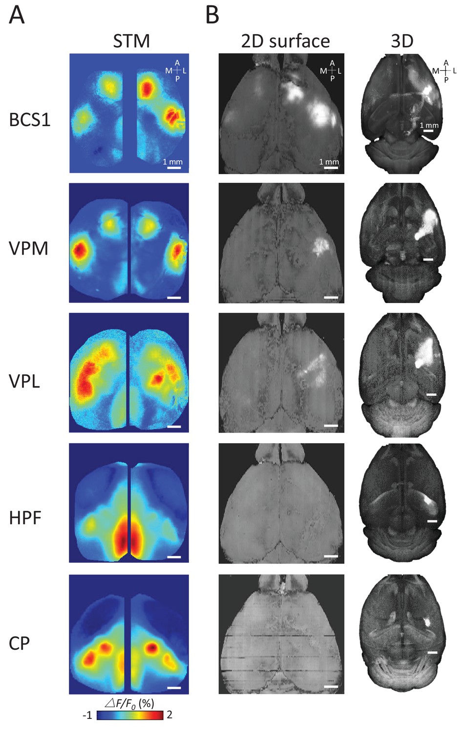
Examples of STMs and projection maps.
(A) Example of STMs from neurons recorded in BCS1, VPM, VPL, HPF and CP. (B) Example of projection maps (2D surface and 3D) reconstructed from Allen Brain Atlas with injection sites (Oh et al., 2014) in the same region as our recording. For example, for a spiking neuron recorded in BCS1 we show anterograde labeling of GFP emanating from an injection site in BCS1 that extends to motor cortex and is present across cortex in the 2D surface plot of cortex. This projection pattern for BCS1 matches the STM map quite well as in previous work (Mohajerani et al., 2013). In contrast, for sub-cortical injections of GFP tracer such as in HPF there was less overlap between STMs and projection maps perhaps indicating polysynaptic pathways. Website: 2015 Allen Institute for Brain Science. Allen Mouse Brain Connectivity Atlas [Internet]. Available from: http://connectivity.brain-map.org.
Figure 6 with 6 supplements
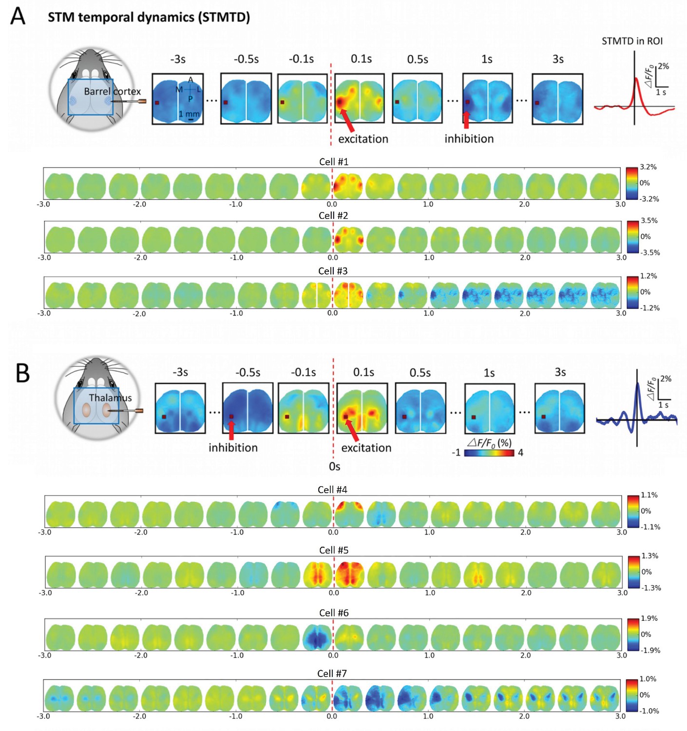
Montages of cortical and thalamic spatio-temporal dynamics.
(A) Top: right hemisphere barrel cortex neuron spiking time montage stereotyped dynamics in left hemisphere barrel cortex region-of-interest (ROI). The maximally activated pixel in the ROI (red arrow) is tracked over time and reveals Spike-Triggered-Map Temporal Dynamics (STMTD) which rises quickly at spike time t = 0 and decays in 100–200 ms followed by 1–2 s cortical depression (red curve in right plot). Bottom: Additional examples of right hemisphere barrel cortex neuron spike-triggered montages show similar barrel-motor cortex activation pattern with peaks in cortical activation shortly following spiking and a return to baseline or prolonged depression. (B) Top: Same as in A, but for a thalamically recorded neuron (right hemisphere) which correlates strongly with motor cortex activation shortly after spiking. Bottom: Additional montage examples of thalamic neurons (also right hemisphere) reveal both the spatial diversity (i.e. different STMs) and temporal diversity (i.e. different STM dynamics).
Figure 6—figure supplement 1
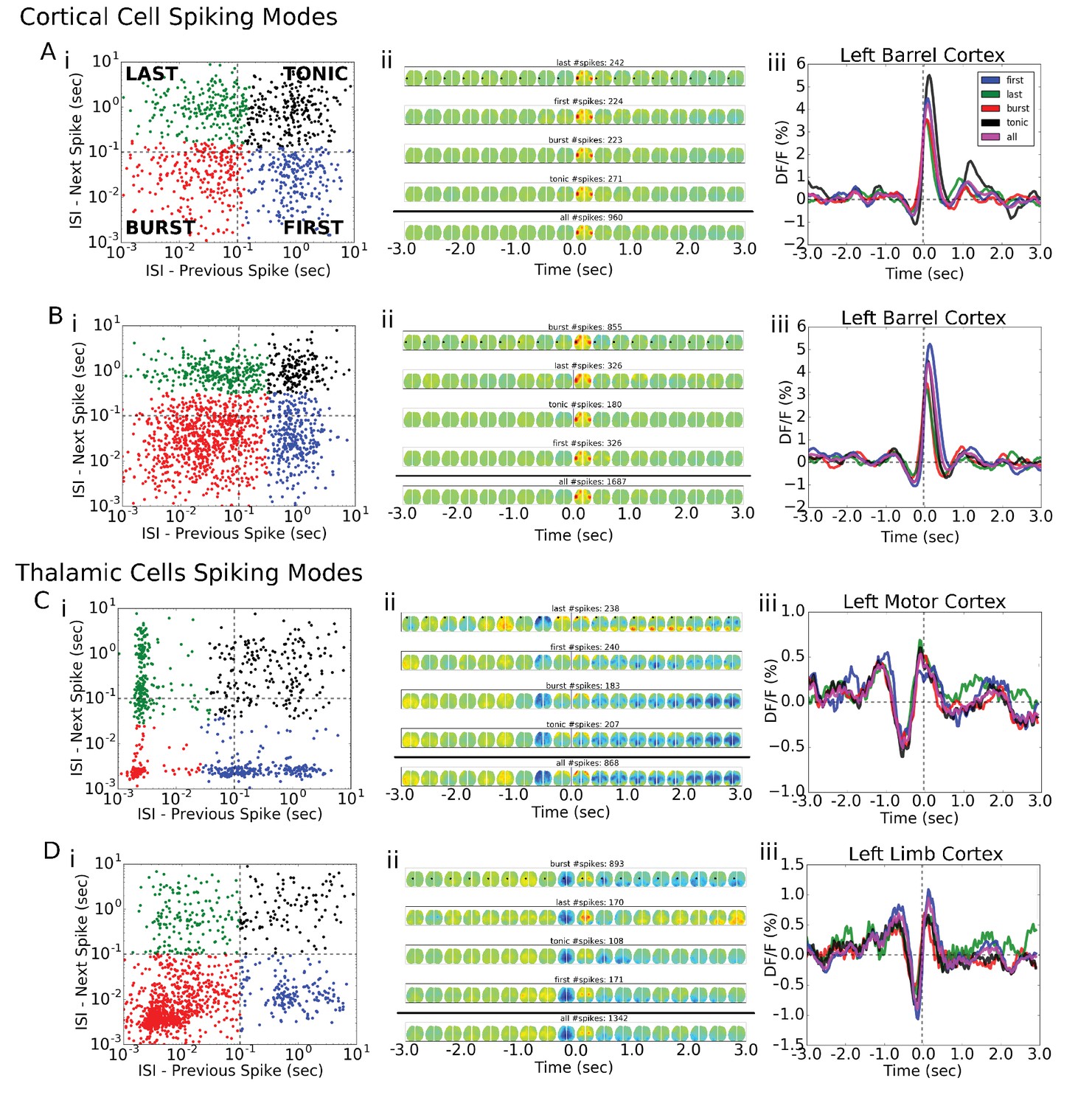
Single-cell STM and STMTDs are similar across spiking modes.
(Ai, Bi) Cortical cell spiking modes determined by grouping the distribution of each spike’s inter-spike-interval between previous (x-axis) and following (y-axis) spike. The four quadrants indicate different firing modes (see Materials and methods). Cortical cells recorded (barrel cortex) did not have clear spiking modes but some clusters were present and spikes were grouped according to those divisions. (Aii, Bi) Six-second motifs generated using spikes from different spiking modes in part (i) are largely the same for cortical cells. (Aiii, Biii) Temporal dynamics of left-hemisphere barrel cortex tracked across time for all spiking modes were largely similar. (Ci, Di) Same as in A, but for thalamic cells where bursting modes are more visible. (Cii, Dii) same as in (Aii). (Ciii) same as (Aiii) with tracking of left-hemisphere motor cortex activity. (Diii) same as (Aiii) but with tracking of left-hemisphere limb cortex activity.
Figure 6—figure supplement 2
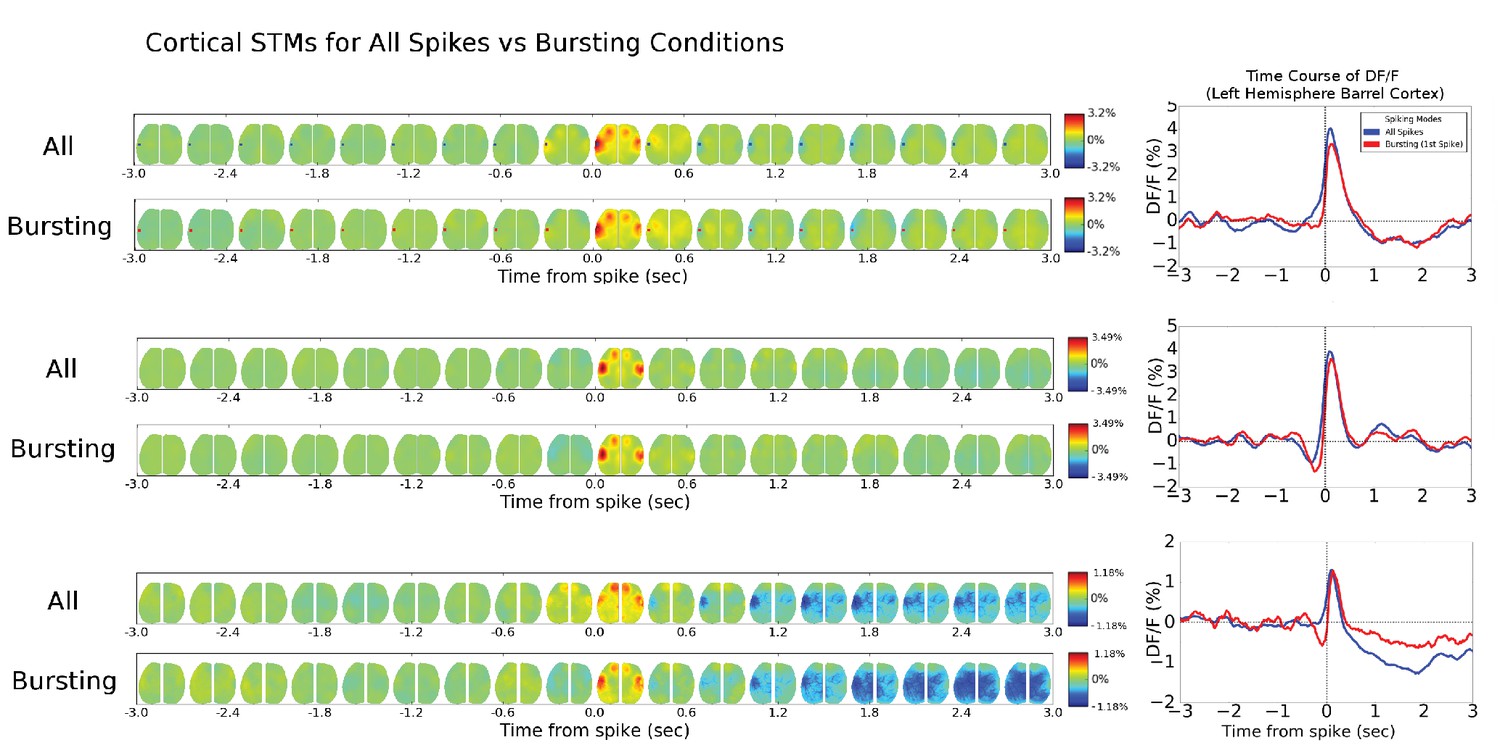
Cortical cell STM and STMTDs are similar across spiking modes.
Left: Spatio-temporal motifs for the three cortical cells presented in Figure 6 considering contributions of all spikes from each cell (top motif) versus just the bursting condition for each cell (i.e. only spikes that are preceded by a >500 ms silent period). Right: The time course of the peak signal in the left hemisphere barrel cortex (see Figure 6 also) for all spikes (blue) and first spikes in a burst (red curves). Both the motifs and time course curves are similar for both conditions.
Figure 6—figure supplement 3
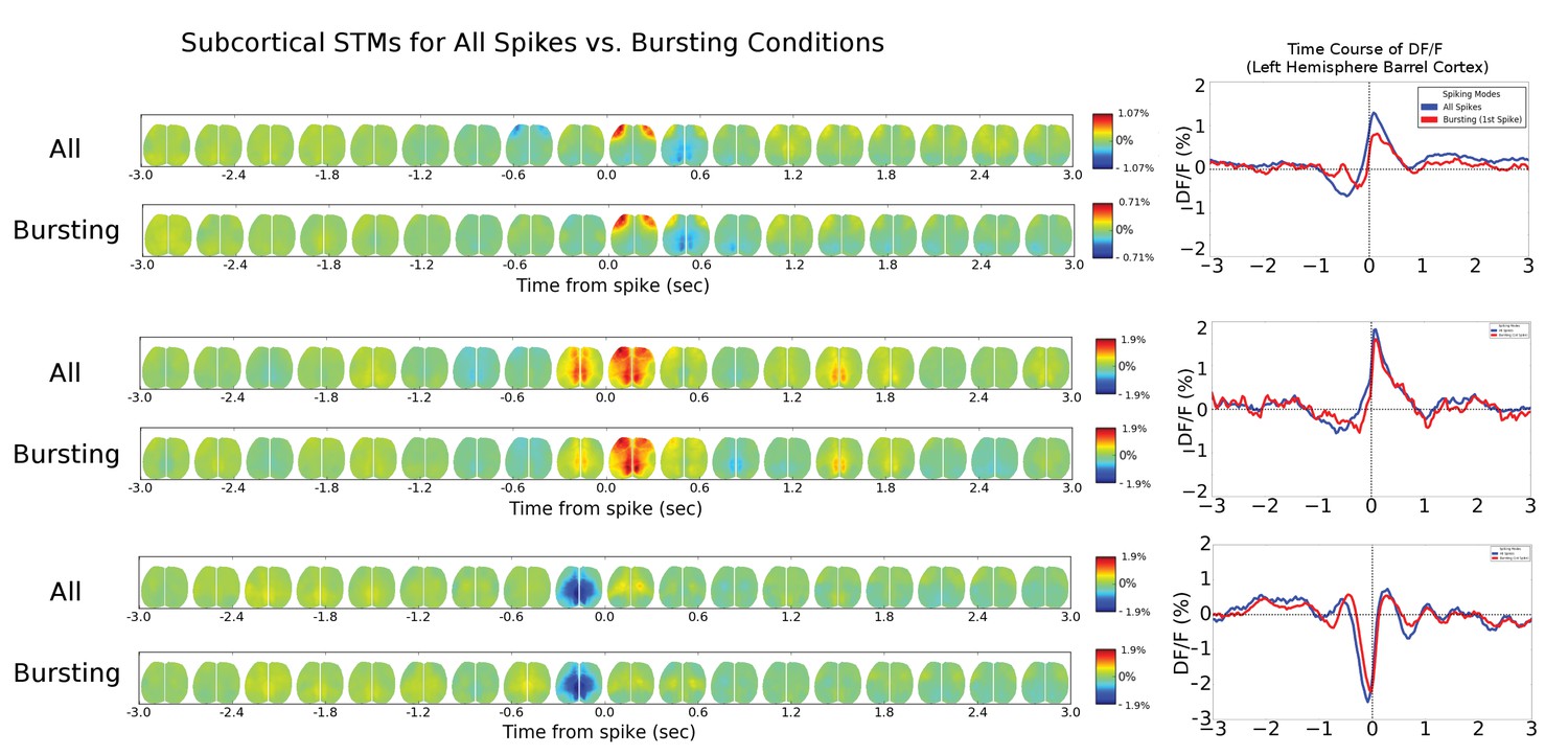
Thalamic cell STM and STMTDs are similar across spiking modes.
Left: Spatio-temporal motifs for the three of the four cortical cells presented in Figure 6 considering contributions of all spikes from each cell (top motif) vs. just the bursting condition for each cell (i.e. only spikes that are preceded by a >500 ms silent period). Right: The time course of the peak signal in the left hemisphere barrel cortex (see Figure 6 also) for all spikes (blue) and first spikes in a burst (red curves). Both the motifs and time course curves are largely the same for both conditions. The bursting condition for the fourth cell in Figure 6 had an STM with a very small and noisy ΔF/F0value (~0.25%) and was excluded from comparison here.
Figure 6—figure supplement 4

Single spike motifs sub-grouping reveals similar STMs across sub-networks.
(A) Five examples of STMs generated from a single spike from a cell reveal substantial variability and high activation (ΔF/F0 >10% for some spikes). (B) Distribution of all single spike STMs (3779 spikes for example cell) from a single cortical cell visualized in two-dimensions using PCA does not reveal natural clusters and is partitioned into four sub-networks (coloured dots) each with a distinct centre (larger colour circles). (C) Spike rasters for the four sub-networks reveal that spikes in each sub-network are distributed in time and that inter-spike-intervals (ISIs) are largely similar for all four sub-networks (green, red, blue and magenta colours) and overall sum (black colour). (D) STMs generated from the four sub-networks reveal substantial differences in the sub-network dynamics (top four STMs) with the sum of all STMs providing the average STM pattern (bottom STM). Note that partitioning the data randomly does not reveal these sub-networks but patterns similar to the total spike STM. (E) Same as (A) but STM examples are from all possible spontaneously occurring motifs during the recording (9439 possible motifs in a ~5.2 mins recording at 30 Hz). (F) Same as in (B) but STM distributions are for all spontaneous motifs – with the centres of the sub-networks obtained from the single-cell motif sub-networks. This results in spontaneous motif sub-networks that are the closest to single-cell generated sub-networks. (G) Same as in (C) but for all spontaneous motifs. The ISI histograms peak at ~33 ms (i.e. single inter-frame-interval) indicates that spontaneous motifs group naturally into sub-networks and are dominated by ‘bursts’ of similar motifs each separated by single frames. (H) Same as in (D) but for the four sub-networks generated from spontaneous motifs. As expected the sum of all spontaneous motifs is ~0.0% ΔF/F0. (I) Subtracting spontaneous motifs from cell generated motifs reveals that single cell STM contribution is largely uniform despite the participation of cell spiking in different sub-networks identified (see D).
Figure 6—figure supplement 5
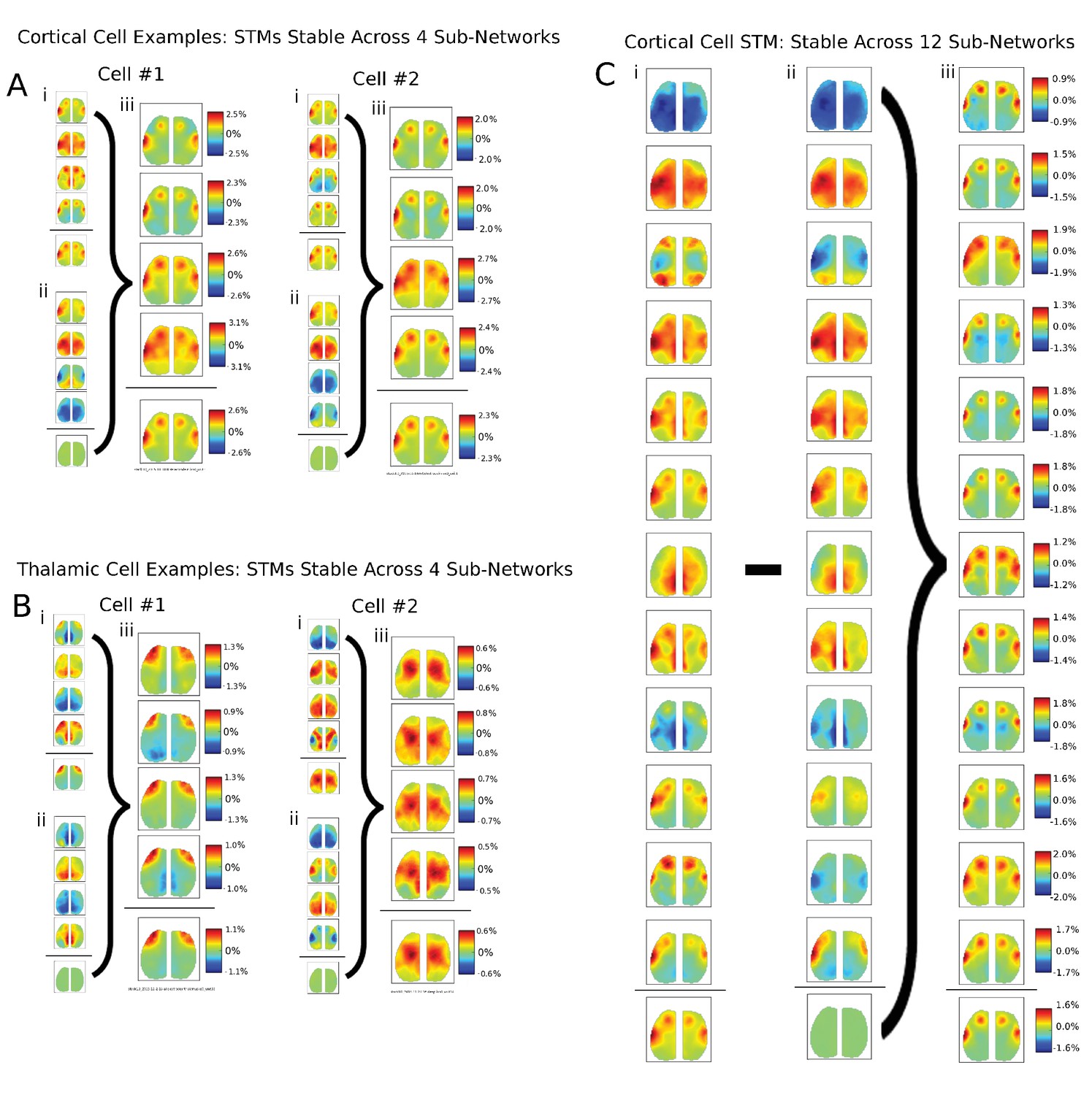
Additional examples of single cells STM stability in other mice and for larger partition sizes.
(A) Two examples of single cortical cell STMs recovered from sub-networks: (i) four spike-triggered sub-network STMs; (ii) spontaneous sub-network STMs; (iii) difference between cell-triggered and spontaneous motifs – reveal single cell contributions to active sub-networks. (B) Same as (A) but for two thalamic cells. (C) Same as in (A) but partitioning data into 12 sub-networks also reveals that average STMs are largely recoverable from active sub-networks.
Figure 6—figure supplement 6
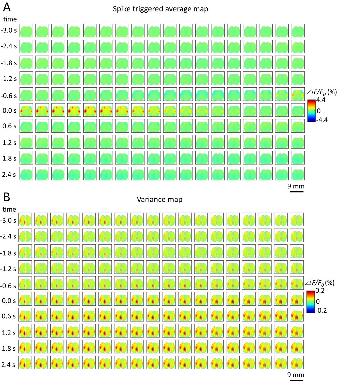
Spike-triggered variance map.
(A) Spatiotemporal dynamic of spike-triggered average map of a cortical neuron. The time window is from −3s to 3s. (B) Spatiotemporal dynamic of spike-triggered variance map of the same neuron. The amplitude of the variance is small (△F/F0 (%) from −0.2 to 0.2).
Figure 7 with 1 supplement
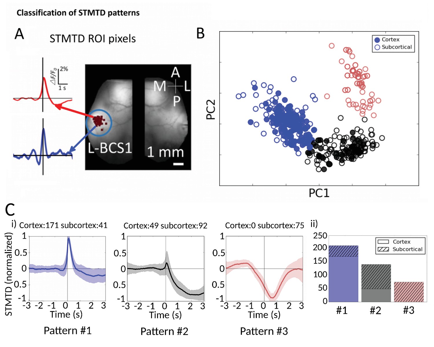
Classification of STMTD patterns.
(A) Example of two STMTDs from pixels within L-BCS1 (left barrel cortex) from a single mouse recording (both cortical and subcortical neurons STMTD pixel locations shown). Each recorded cell STMTD has a slightly different maximum pixel amplitude location, but all fall within the L-BCS1 region. (B) STMTD PCA distribution from all 428 cortical and subcortical neurons recorded from all mice separated using KMEANS (k = 3). (Ci) STMTD patterns (±SD) classifications from (B). The number of neurons from cortex and thalamus used for the average are presented in title. (ii) Distribution of STMTD classification between cortical (clear) and subcortical (hashed) neuron generated STMTDs.
-
Figure 7—source data 1
Data files for PCA distribution clusters.
This zip archive contains all original STMTDs (*traces.txt files) from cortical cells (220) and subcortical cells (208) used in generating Figure 7B. The STMTDs are interpolated to 100 Hz (i.e. 600 time points for each cell for a 6 s period). The archive also contains (3D) coordinates from PCA distributions of the traces (*scatter.txt files) which are displayed in Figure 7B. Both traces and PCA coordinates can be viewed independently.
- https://doi.org/10.7554/eLife.19976.020
Figure 7—figure supplement 1
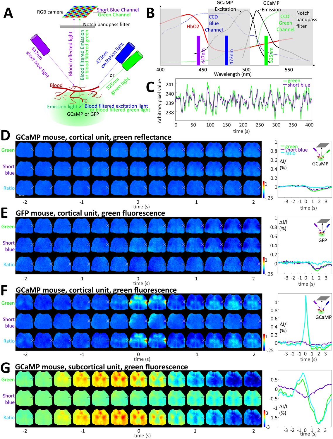
Limited contribution of blood artifacts on STA.
(A) Diagram of the experimental setup used to evaluate the contribution of blood volume to the GCaMP green fluorescence. Local blood volume was evaluated by measuring the change in short blue (447 nm) and green reflectance (525 nm, for validation control only, see panel B) while hemoglobin is known to absorb blue and green light. Green fluorescence of GFP or GCaMP was excited by using 473 nm excitation light when 525 nm light was turned-off (and 447 nm light turned-on). Short blue reflectance and green reflectance or fluorescence was imaged using a RGB color camera. (B) Spectrum of excitation and emission of GCaMP (black curves, similar for GFP) and absorption of hemoglobin (red). The transmission of the blue and green channel depends of the window of the triple band-pass filter (dash gray boxes) and the transmission of the blue and green channels of the CCD camera (dotted blue and green curves). (C) Spontaneous activity of green and short blue reflectance (cross-correlation: r = 0.93). Blue channel DC was adjusted to fit with green channel baseline and both channels were low-pass filtered (0.033 Hz). (D) First and Second lines: cortical STA generated from green reflectance (using green LED) and short blue reflectance (using short blue LED) from a GCaMP mouse. Third line: Ratio of the two STAs green over short blue. Left: STA values within BCS1 for green and short blue channels (cross-correlation: r = 0.88 ± 0.04, n = 7; present example: r = 0.92) as well as ratio. (E) First and Second lines: cortical STA generated from GFP fluorescence (using blue LED) and short blue reflectance (using short blue LED) from a GFP mouse. Third line: Ratio of the two STAs green over short blue. (F,G) Same as C but for a GCaMP mouse and for cortical and subcortical STA.
Figure 8 with 1 supplement

Spatiotemporal patterns of STMs.
(A) Top: Normalized STMTDs (as in Figure 7) from maximum pixels tracked in multiple ROIs (HLS1, FLS1, BCS1, RS, V1, M1, PTA and ACC, see Table 1) for 255 cortical cells. Each horizontal line represents a single neuron's STMTD in each of the eight ROIs considered normalized to that neuron's STMTD maximum or minimum activation. Bottom: average and standard deviation of STMTD within each ROI for all cells. (B) Same as A, but for all thalamic neuron generated STMTDs. The thalamic STMTDs are more diverse, less temporally precise, and contain longer depression epochs – revealing ROI specificity and cortical vs. subcortical differences. These results are from awake mice.
Figure 8—figure supplement 1

Limited contribution of body movement on STA.
(A) Image insets: pictures of the frame average and standard deviation showing the location of movement over one entire recording. Yellow box: region of interest used to quantify movement. Graph: Black curve is movement density calculated for each frame by measuring the average of absolute gradient within the region of interest (yellow box). Standard deviation (σ) and median of the profile were calculated and period of quietness and movement are identified by selecting periods of time below [median+σ/10] (green) and above [median+σ] (red), respectively. (B) STA generated for all spikes (top, black curve) and spike restricted to period of quietness (bottom, green curve). (C) Maximum and positive peaks amplitude for STA from all and quietness period only spikes showing no change (paired t-test: p=0.108 and 0.431, respectively, n = 31).
Author response image 1
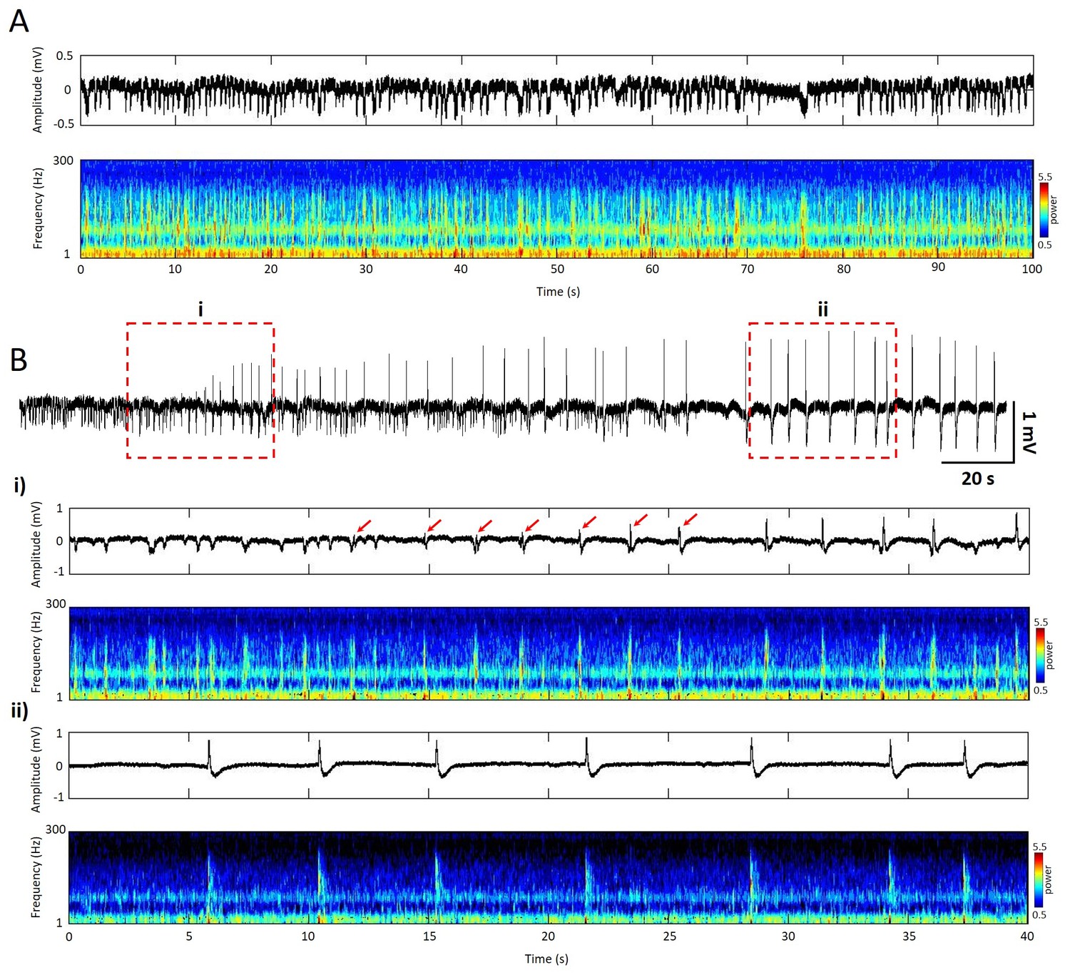
Temporal and spectral signatures of spontaneous and epileptic events measured from the local field potential (LFP).
(A) Top (black trace), 100s segment of LFP recording of spontaneous activity from superficial layer of cortex. Bottom, spectrogram (Morlet-wavelet scalograms) of the LFP trace. (B) Top (black trace), 170s segment of LFP recording after application of Picrotoxin (Sigma) on the top of cortical surface during the same experiment. (i) Top (black trace), 40s segment of LFP recording, epileptic events initiated with reversed phase and gradually increased amplitude (red arrows). Bottom, spectrogram of the LFP trace. (ii) Top (black trace), 40s segment of LFP recording showed repetitive high amplitude (>1 mV) epileptic discharge. Bottom, spectrogram showed high frequency power during the epileptic events but suppressed background activity.
Author response image 2
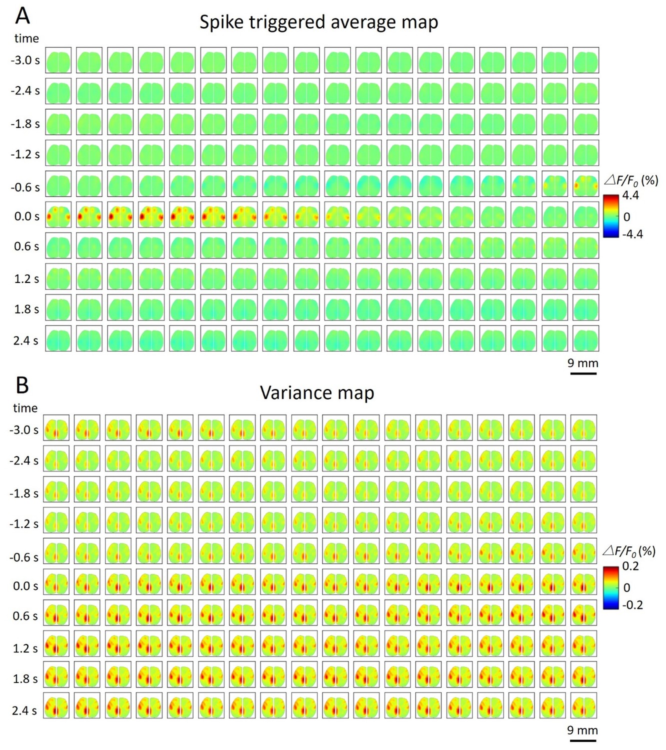
Spike-triggered variance map.
https://doi.org/10.7554/eLife.19976.030
Author response image 3

Spike Triggered Covariance Analysis of BCS1 Neuron.
(A) Each calcium image was recorded each Δt = 33.33 ms (frame rate = 30 Hz), and the spikes recorded in BCS1 neuron were binned within the same interval. In this example, we recorded 15250 frames and 4625 spikes simultaneously. (B) We constructed the covariance matrix of the spatiotemporal calcium images, followed by eigenvector analysis of the covariance matrix and plotted its spectrum (black). We compared this spectrum to that expected theoretically for the same-sized random matrix (red). (C) PCA of calcium images covariance matrix. The eigenvectors of the calcium images covariance matrix that correspond to the largest eigenvalues (mode 1 to 12) are seen to contain sequence of spatiotemporal patterns. (D) Spatiotemporal dynamic of STA map for cell #1 and cell#2. Calcium images were binned from 128*128 to 32*32 square pixel array with mask to select brain region. (E) Distribution of underlying calcium image matrix projected on Spike triggered average (STA) for cell #1 and cell #2. (F) The input/output nonlinearity of cell #1 and cell#2, input project on STA (S*sta).
Author response image 4

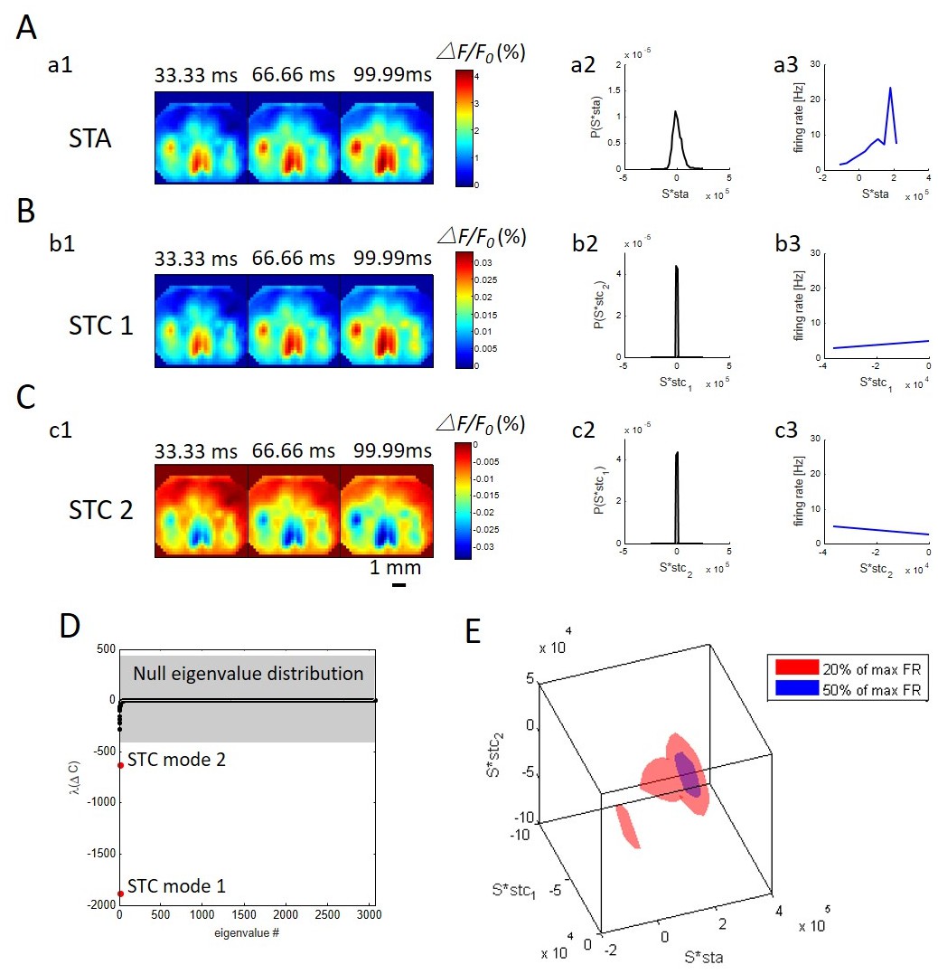
Spike Triggered Covariance Analysis of sub-cortical Neuron.
(A) a1. STA of this sub-cortical neuron shows unique spatiotemporal pattern. a2. Distribution of underlying calcium image matrix projected on STA of this sub-cortical neuron. a3. The input/output nonlinearity of this neuron, input project on STA (S*sta). (B) b1. Spike triggered covariance mode 1 (STC1) of this neuron. b2. Distribution of underlying calcium image matrix projected on STC1. b3. The input/output nonlinearity of this neuron, input project on STC1 (S*stc1). (C) c1. Spike triggered covariance mode 2 (STC2) of this neuron. c2. Distribution of underlying calcium image matrix projected on STC2. c3. The input/output nonlinearity of this neuron, input project on STC2 (S*stc2). (D) The significance of each candidate STC feature, were determined by comparing the corresponding eigenvalue (red and black) to the null distribution (gray shaded area). We used 1,000 repetitions of the calculation for randomized spike trains, corresponding to a confidence level of 0.05. (E) Three dimensional plot of the nonlinearity in the space, spanned by the STA and other two orthogonalized STC feature, with surfaces for firing rates (FR) equal to 20% and 50% of the max.
Author response image 5
Running median and random spike normalization.
(A) STA from real spikes (1st line), random spikes (2nd line) and real spikes after running median filtering (3rd line). 4th and 5th lines are subtractions of STA by random spikes and running median respectively. (B) STA dynamic within BCS1 for real spikes (black curve), random spikes (thin red) and the subtraction (Thick red). (C) Same as B but for running median. (D,E) While drift was not often observed it was artificially introduced by reducing the DC of spontaneous activity by 50% in 9min. Both subtractions (random spikes and running median) were able to remove the slow drift contribution. However, post-spike depression (black arrow) at ∼1s was only preserved by using random spikes correction.
Videos
Video 1
Cortical neuron-triggered bilateral mesoscale calcium activity.
Left: dorsal cortex calcium dynamics triggered from a right hemisphere barrel cortex recorded cell. Right, time-course reflecting dynamics in the left hemisphere barrel cortex (green) alongside a lower activated area (red). Dynamics in region-of-interest (green) exhibit high activation correlating with spiking time (t = 0 s) followed by a 2 s depression in fluorescence signal. Activity illustrated 3 s prior to, and 3 s following cell spiking.
Video 2
Thalamic neuron #1 triggered bilateral mesoscale calcium activity.
As in Video 1 but from a right-hemisphere thalamic neuron. Region-of-interest (green) in the left hemisphere exhibits a transient pre-spiking depression followed by activation correlating with spike timing.
Video 3
Thalamic neuron #2 triggered bilateral mesoscale calcium activity.
As in Video 2 but from another thalamic neuron revealing peak activation in a different region-of-interest.
Video 4
Thalamic neuron #3 triggered bilateral mesoscale calcium activity.
As in Video 2. Depressed cortical calcium activity is present in the left hemisphere barrel cortex region-of-interest prior to spiking and persists for an additional 2 s.
Video 5
Evaluation of whisker movement.
Left: Average of absolute gradient within the region of interest (yellow box in Figure 8—figure supplement 1) between the frames 3400 and 5000. Right: Corresponding image frames displayed at real time.
Tables
Table 1
Abbreviation used to define different cortical/sub-cortical areas.
S1 | Primary somatosensory area |
|---|---|
S2 | Supplemental or Secondary Somatosensory area |
FL | Forelimb region of the Primary Somatosensory area (FLS1) |
HL | Hindlimb region of the Primary Somatosensory area (HLS1) |
BC | Barrel region of the Primary Somatosensory area (BCS1) |
M1 | Primary motor area |
M2 | Secondary motor area |
MO | Mouth region of the Primary Somatosensory area |
NO | Nose region of the Primary Somatosensory area |
TR | Trunk region of the Primary Somatosensory area |
UN | (Unassigned) region of the Primary Somatosensory area (S1) |
AC | Anterior Cingulate area (ACC) |
A | Anterior or Posterior Partial Association areas: PTLp or PTA |
V1 | Primary visual cortex |
AL | AnteroLateral regions of the extrastriate visual areas |
AM | AnteroMedial regions of the extrastriate visual areas |
LM | LateralMedial regions of the extrastriate visual areas |
PL | PosteroLateral regions of the extrastriate visual areas |
LI | LateralIntermediate regions of the extrastriate visual areas |
PM | PosteroMedial regions of the extrastriate visual areas |
POR | Postrhinal regions of the extrastriate visual areas |
RL | RostroLateral regions of the extrastriate visual areas |
AU | Primary Auditory area |
TEA | Temporal Association area |
RS | Retrosplenial area |
PTA | Parietal Association area |
VPM | Ventral posteromedial nucleus of the thalamus |
VPL | Ventral posterolateral nucleus of the thalamus |
PO | Posterior complex of the thalamus |
RT | Reticular nucleus of the thalamus |
LGN | Lateral geniculate nucleus |
CP | Caudoputamen |
HPF | Hippocampal formation |
Download links
A two-part list of links to download the article, or parts of the article, in various formats.
Downloads (link to download the article as PDF)
Open citations (links to open the citations from this article in various online reference manager services)
Cite this article (links to download the citations from this article in formats compatible with various reference manager tools)
Mapping cortical mesoscopic networks of single spiking cortical or sub-cortical neurons
eLife 6:e19976.
https://doi.org/10.7554/eLife.19976


