A general method for determining secondary active transporter substrate stoichiometry
- National Institute of Neurological Disorders and Stroke, National Institutes of Health, United States
Figures
Figure 1
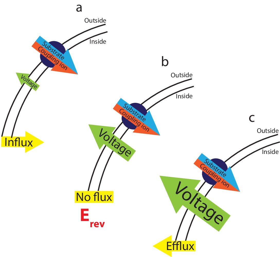
The interplay between substrate gradients, the membrane potential and flux.
Electrogenic transporters cause charge build up across the membrane, which inhibits further transport. The combined gradients of coupling ion and substrate (illustrated here for a symporter with red/blue arrow), and the applied membrane potential (voltage, green arrow) therefore influence the direction of substrate flux across the membrane. Depending on the magnitude of these opposing forces, three outcomes can occur: (a) at applied voltages that are insufficient to oppose the diffusional force of the substrates, influx of substrate occurs. (b) At the equilibrium, or reversal, potential, Erev, the applied voltage exactly opposes the diffusional force of the substrates resulting in no net flux. (c) At higher applied voltages, the voltage overcomes the electrochemical gradient imposed by the coupling ion and substrate gradients, reversing the direction of flux and efflux occurs.
Figure 2

Direction of substrate flux can be controlled by the magnitude of the membrane potential.
(a) Schematic of experimental conditions with outwardly directed [3H]-succinate gradient (red arrow) and inwardly directed Na+ gradient (blue arrow) in proteoliposomes containing VcINDY. While the succinate and Na+ gradients are kept constant, the K+ gradient (orange arrow) was varied (‘V’) in the presence of valinomycin (Val.) to set the membrane potential. The direction of the arrow indicates the direction of the gradient. (b) Internalized [3H]-succinate (CPM) measured over time in the presence of three applied voltages; 12 mV (red), 48 mV (blue), and 84 mV (green). The yellow datapoint indicates the level of internal [3H]-succinate prior to start of the reaction. Grey dashed line indicates the initial level of internal counts. Exact buffer conditions are detailed in Supplementary file 1. Triplicate datasets are shown and error bars represent S.E.M. This experiment was reproduced on three separate occasions.
Figure 3 with 1 supplement
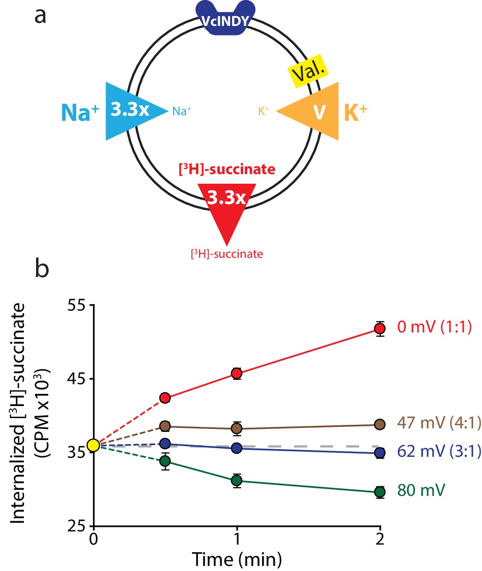
Reversal potential for VcINDY transport suggests a 3:1 coupling stoichiometry.
(a) Schematic describing experimental conditions as in Figure 2a. (b) Internalized [3H]-succinate (CPM) over time in the presence of four different voltages: 0 mV (red), 47 mV (brown), 62 mV (blue), and 80 mV (green). The coupling stoichiometry (Na+:succinate2-) for each possible reversal potential is shown in parentheses for each applied voltage. The 80 mV condition, which is not the calculated reversal potential for any candidate coupling stoichiometry, serves as a proof of flux reversal. Grey dashed line indicates the initial level of internal counts. The exact buffer conditions used in this experiment are detailed in Supplementary file 1. Each experiment was performed in triplicate and error bars represent S.E.M. This experiment was performed on three occasions and found to be reproducible.
Figure 3—figure supplement 1
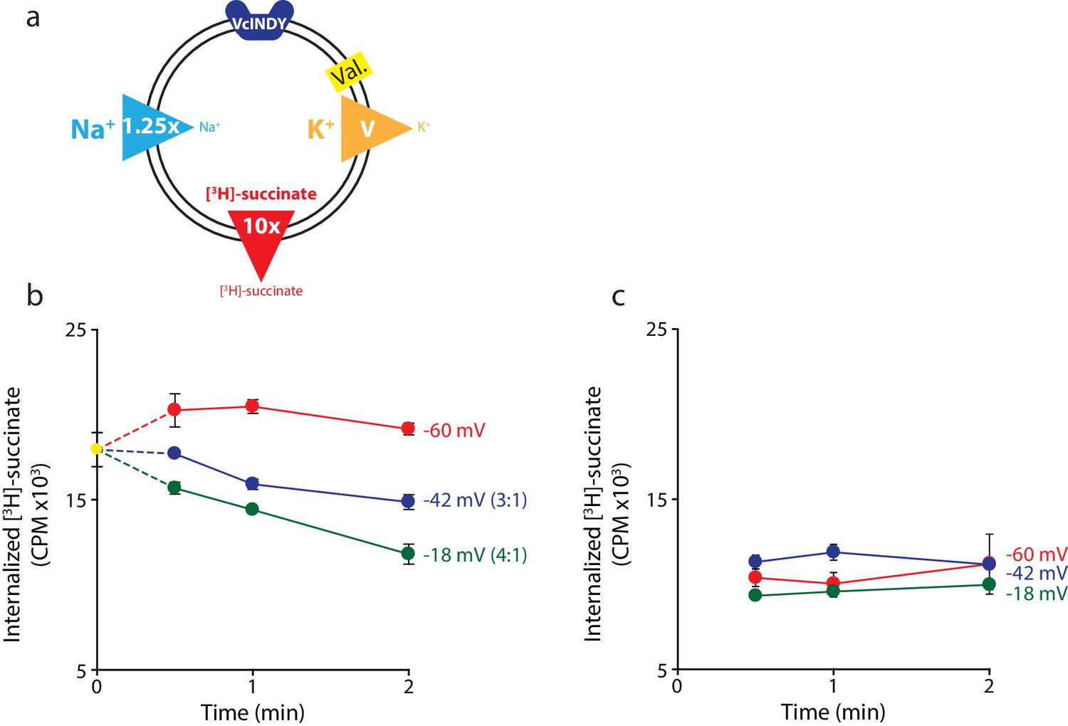
Negative membrane potentials suggest a 3:1 coupling stoichiometry for VcINDY.
(a) Schematic describing experimental conditions as in Figure 2a. (b) Internalized [3H]-succinate measured as a function of time in the presence of three different negative membrane potentials: −60 mV (red), −42 mV (blue), and −18 mV (green). Exact buffer conditions are detailed in Supplementary file 1. The coupling stoichiometry (Na+:succinate2-) for each possible reversal potential is shown in parentheses for each applied voltage. The −60 mV condition served as the proof of flux reversal. (c) The same experiment as in (b) except with protein-free liposomes. Triplicate datasets are shown and the error bars represent S.E.M. The experiment in (b) was reproduced on two separate occasions and the experiment in (c) was performed once.
Figure 4 with 1 supplement

Voltage-ΔCPM plot of VcINDY transport for three different sets of substrate and coupling ion gradients.
ΔCPM for three sets of gradients plotted as a function of voltage. ΔCPM values were calculated by subtracting the CPM at 1 min (green and blues traces) and 30 s (red trace) from the initial counts for each voltage tested (Green data from Figure 2, Blue data from Figure 3, Red data from Figure 3—figure supplement 1). The reversal potentials for each gradient set are indicated by the dashed line and each represents a 3:1 coupling stoichiometry. Triplicate data sets are shown and error bars represent S.E.M.
Figure 4—figure supplement 1
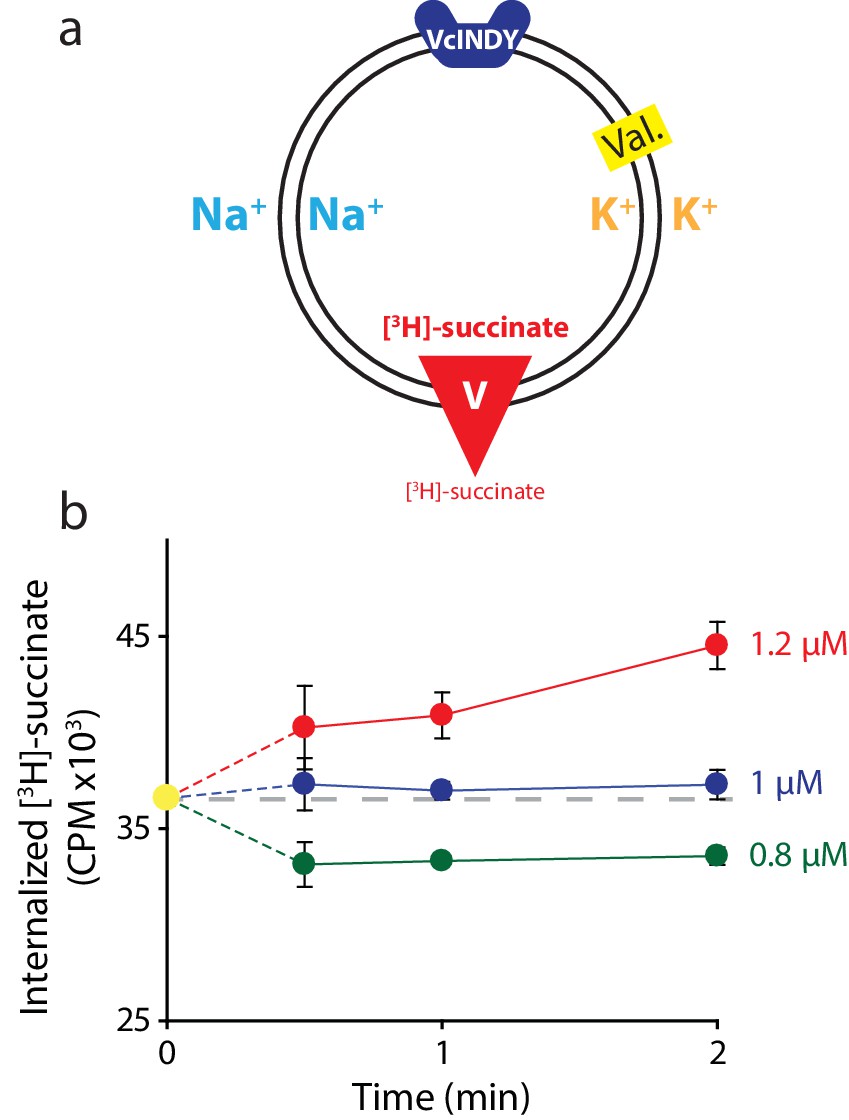
Determining the internal concentration of succinate using flux equilibrium.
(a) Schematic describing experimental conditions as in Figure 2a. Here, equal concentrations of Na+ and K+ are present on both sides of the membrane and substrate is varied (V). The membrane potential is clamped at 0 mV. (b) Internalized [3H]-succinate measured as a function of time in the presence of three different concentrations of external succinate: 1.2 μM (red), 1 μM (blue), and 0.8 μM (green). Triplicate datasets are shown and error bars represent S.E.M. This experiment was on a single occasion.
Figure 5
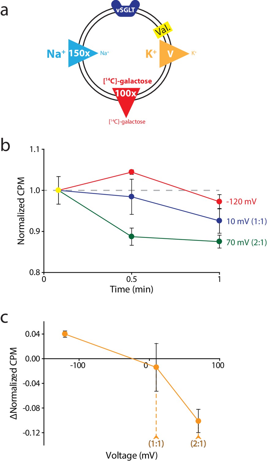
Reversal potential for vSGLT transport indicates a 1:1 coupling stoichiometry.
(a) Schematic describing experimental conditions as in Figure 2a., except with an outwardly directed [14C]-galactose gradient instead of succinate. (b) Internalized [14C]-galactose measured over time in the presence of three different voltages: −120 mV (red), 10 mV (blue), and 70 mV (green). The exact buffer conditions used in this experiment are detailed in Supplementary file 1. (c) Voltage-ΔCPM plot of the data in part (b). ΔCPM was calculated by subtracting the CPM values at 30 s from the normalized y-intercept. Numbers in parentheses represent coupling stoichiometry (Na+:galactose) for each membrane potential. Triplicate datasets are shown and the error bars represent S.E.M. This experiment was reproduced on two separate occasions.
Additional files
-
Supplementary file 1
Exact buffer conditions for all experiments presented.
Constituent concentrations of internal and external buffers used in each experiment. ICD stands for internal concentration determination. Columns are color-coded to match the experimental schematics presented in each figure.
- https://doi.org/10.7554/eLife.21016.009
Download links
A two-part list of links to download the article, or parts of the article, in various formats.
Downloads (link to download the article as PDF)
Open citations (links to open the citations from this article in various online reference manager services)
Cite this article (links to download the citations from this article in formats compatible with various reference manager tools)
A general method for determining secondary active transporter substrate stoichiometry
eLife 6:e21016.
https://doi.org/10.7554/eLife.21016


