Calcium dynamics regulating the timing of decision-making in C. elegans
- Osaka University, Japan
- Tohoku Bunka Gakuen University, Japan
- The University of Edinburgh, United Kingdom
- Saitama University, Japan
- The University of Tokyo, Japan
- Ibaraki University, Japan
- Tohoku University, Japan
Figures
Figure 1 with 1 supplement
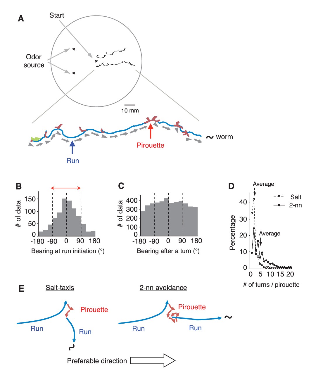
C.elegans selectively initiates runs away from the odor source.
(A) Examples of the tracks of 2 animals during 12 min of 2-nonanone avoidance assay, overlaid on a schematic drawing of a 9 cm plate. One of the tracks is magnified below. In the magnified view, pirouettes are red and runs are blue. Arrow heads and arrows indicate the directions of run initiation and those during runs, respectively. (B) Histogram indicates the bearings at run initiation during 2-nonanone avoidance (i.e., the bearing of the arrow heads in panel A, and the initial bearing of the blue arrows in panel E). The bearing was determined as B = 0° when animals migrated directly away from the odor source (= down the gradient) and ±180° when they migrated directly toward the source (= up the gradient). Migration away from the odor source (i.e., within ±90° bearings; red arrow) comprised 78.4% of all data. (C) Histogram indicates all the bearings after a turn during pirouettes, including those that later switched to runs (i.e., the initial bearings of the red plus blue arrows in panel E). (D) Percentages of turn numbers per pirouette during 2-nonanone avoidance (solid line and filled circles) and in salt-taxis (dashed lines and open circles). The average number of turns in a pirouette was significantly larger during 2-nonanone avoidance than in salt-taxis (5.2 vs. 2.2 indicated by arrows, respectively; p<0.001 by Mann-Whitney test). (E) Schematic drawings of salt-taxis and 2-nonanone avoidance. Typical chemotaxis such as salt-taxis in C. elegans is regulated by the pirouette (i.e., biased random walk) strategy, where the animal initiates runs mostly in a random direction after a pirouette (Pierce-Shimomura et al., 1999). In contrast, in 2-nonanone avoidance, an appropriate migratory direction is chosen from multiple trials in a pirouette. We refer to this as the ‘pivot-and-go’ strategy. All the statistical details are shown in Supplementary file 1. For panels B, C and D (2-nonanone avoidance), the data are from 100 wild-type animals. Panel D (salt-taxis) is from 64 wild-type animals. The following figure supplement is available for Figure 1.
Figure 1—figure supplement 1

Differences between 2-nonanone avoidance behavior and salt-taxis of C.elegans.
(A) Pirouettes and runs were classified by the length of turn interval (i.e., migratory durations). A distribution of turn intervals during the odor avoidance was fitted by the sum of two exponentials, suggesting that turn interval is regulated by two probabilistic mechanisms (Pierce-Shimomura et al., 1999). Each exponential is indicated by a dashed line, and the sum is indicated by a solid line. The fitted lines were calculated with the least squares method. The vertical axis is a logarithmic scale. A period at which the numbers of the short and long intervals were equal was determined as a threshold value tcrit (vertical red dotted line). Turn intervals longer than tcrit were classified as runs, and shorter intervals and turns were classified in pirouettes. (B) The histogram indicates the bearing in each step (i.e., per second) of the runs during 2-nonanone avoidance. Migration away from the odor source (i.e., within ±90° bearings; red arrow) comprised 83.5% of all data. (C) A typical track of C. elegans during salt-taxis for 20 min (200 mM NaCl spotted onto grid points) (Iino and Yoshida, 2009). As in Figure 1A, pirouettes and runs are indicated with red and blue, respectively. (D) Histogram indicates bearings at run initiation of 64 animals during salt-taxis. In this experiment, the bearing was determined as B = 0° when animals migrated directly toward the source (up the gradient) and ±180° when they migrated directly away from the source (down the gradient). Migration toward the source (i.e., the data within ±90°, indicated by a red arrow) was 59.3% of all data. (E) A distribution of turn interval during the 180 s down phase of the odor gradient (data from Figure 4B, middle right panel) was fitted by the sum of two exponentials similarly to panel A. The fitted lines were calculated with the least squares method.
Figure 2 with 1 supplement
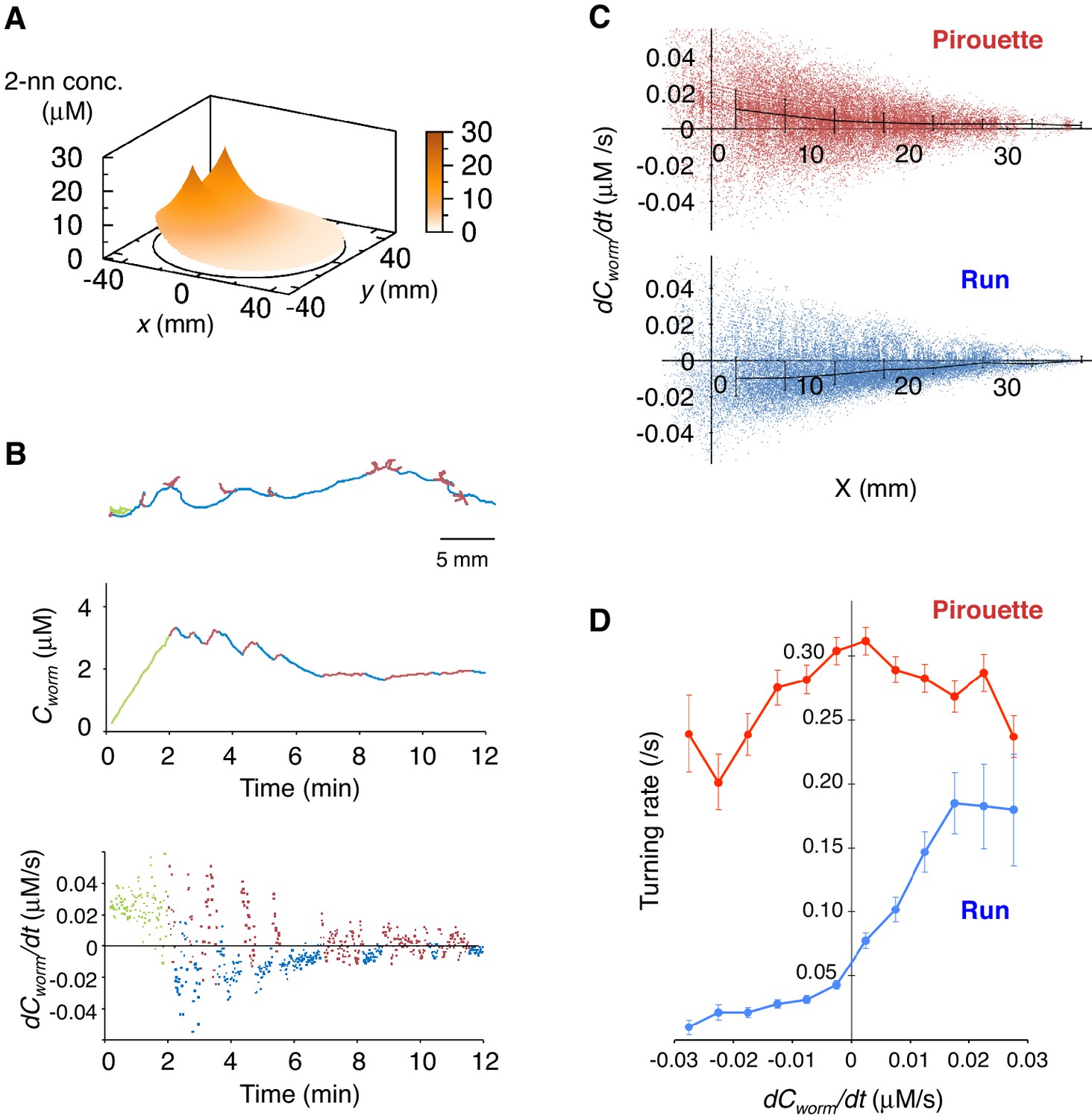
Pirouettes and runs are distinct behavioral states, which are associated with positive and negative dCworm/dt, respectively.
(A) Fitted odor gradient over the assay plate at 12 min, based on the actual measurements shown in Figure 2—figure supplement 1D. (B) (Top) Same with the magnified view of an animal's trajectory in Figure 1A. (Middle, bottom) Graphs showing the 2-nonanone concentration (Cworm: middle) or temporal changes in it (dCworm/dt: bottom) at this animal's position at each second during the odor avoidance behavior. As in Figure 1A, pirouettes and runs are red and blue, respectively. Most of the animals did not migrate much during the first 2 min and were excluded from the analysis (green) because of the rapid increases in the odor concentration during this period. See also Figure 2—figure supplement 1E for another example. (C) Correlation between dCworm/dt and pirouettes or runs. dCworm/dt of 2-nonanone was plotted against the animal's x position for each second during pirouettes (top) or runs (bottom). The bars represent the median ± quartiles for each 5 mm fraction. (D) The responsiveness to the instantaneous dCworm/dt differed between pirouettes and runs. The turning rate was determined as the relationship between dCworm/dt during one second of migration and the probability of turning in the next second. Average turning rates ± SEM for every 0.005 μM/s bin during pirouettes (red line) or runs (blue line) are shown. The data in panels C and D are from the same 100 wild-type animals as in Figure 1. The following figure supplement is available for Figure 2.
Figure 2—figure supplement 1
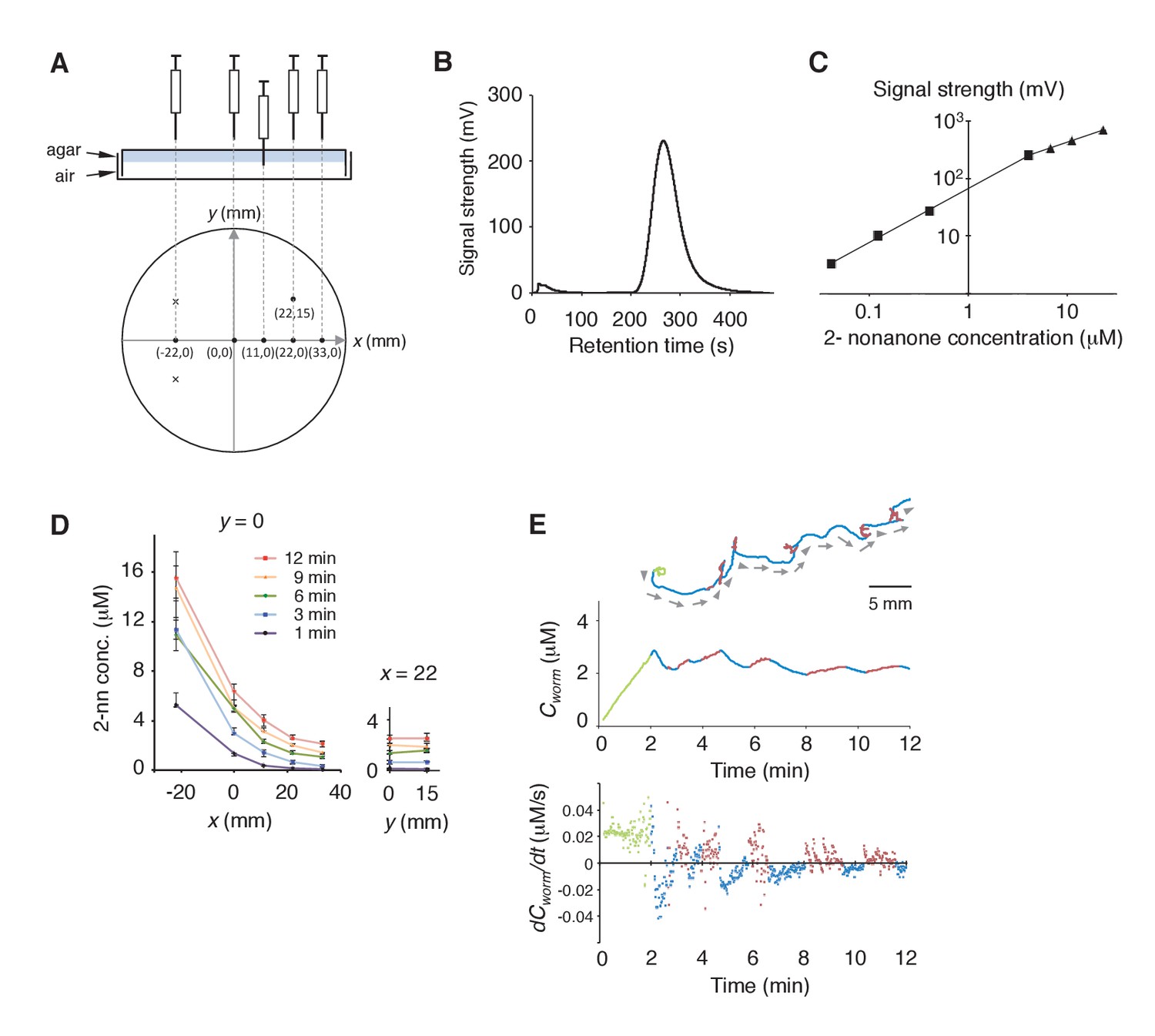
Measurement of the gaseous 2-nonanone gradient in the plate assay paradigm.
(A) A schematic cross-section (upper panel) and top view (lower panel) of gas sampling. The plate is placed upside-down. In the lower panel, crosses indicate positions of the odor source and dots indicate sampling positions, where numbers represent x-y coordinates. In all positions, the tip of the needle was placed ~2 mm below the surface of the agar; an example of the sampling from (x, y) = (11, 0) is shown in the upper panel. The gas sample was immediately subjected to gas chromatography (GC) analysis. Note that one plate was used for each sampling so that sampling did not disturb the odor gradient. (B) A sample record from the GC analysis of 4 μM 2-nonanone. A single large peak was detected at ~260 s, and the peak height was used for calibration. (C) Calibration curve for 2-nonanone. Each dot represents the average of 3–4 experiments, and data on the log-log plot were fit by two simple regression lines for lower (squares) and higher (triangles) concentrations because of the detector's characteristics (see Materials and Methods). (D) 2-nonanone gradient measured along the x axis (left panel) or at (x, y) = (22, 0) and (22, 15) (right panel) at different periods of the assay. The sampling points are indicated in panel A. The gas (0.2 mL) was sampled at 1, 3, 6, 9, and 12 min. Each data point represents the median ± quartile of 7–9 independent experiments. Notably, the error bar of each measured value was small in the right half of the plate (x ≥ 0), where most of the animals were located during the avoidance behavior. This was likely due to the fact that odor diffusion smooths out positional differences in odor concentration. No significant differences were observed along the y axis at the same time point (right panel; Mann-Whitney test). (E) Another example (the upper animal in the top panel of Figure 1A) of correlations between an animal's behavioral pattern and changes in 2-nonanone concentration.
Figure 3 with 1 supplement
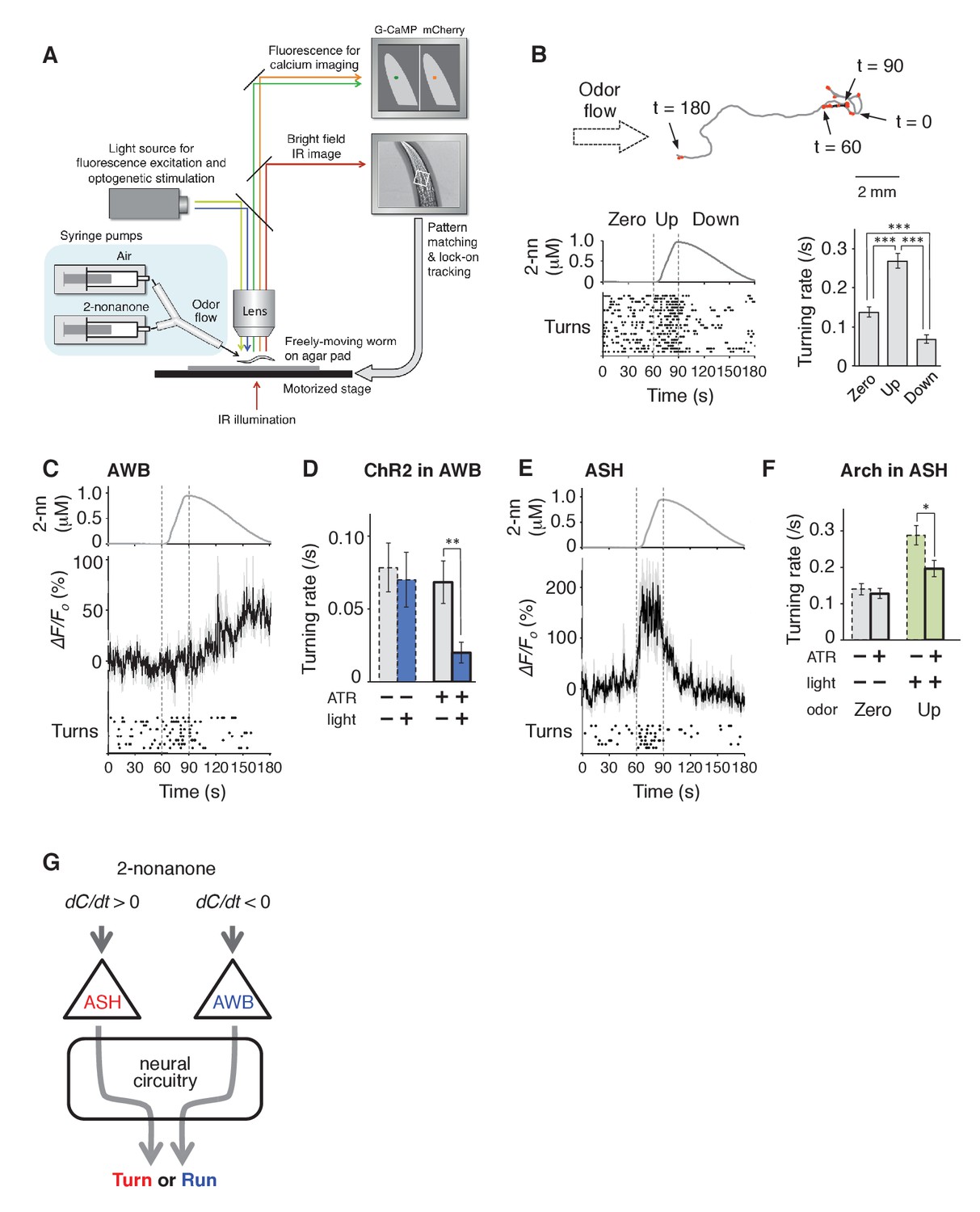
AWB and ASH sensory neuron pairs regulate turning rate in response to dC/dt of 2-nonanone.
(A) Schematic drawing of the OSB2 system. (B) Behavioral response to temporal changes in the 2-nonanone concentration. (Top) Track of a wild-type animal. The first 60 s (gray) is a period of no odor (‘odor-zero phase’ in the bottom left panel), 60–90 s (black) is a period with a constant increase in odor concentration from 0 to 1 μM (‘odor-up phase’), and 90–180 s (gray) is a period with a constant decrease in odor concentration from 1 to 0 μM (‘odor-down phase’). Red dots indicate turns. (Bottom left) Rastergram of turns. The upper portion of the panel shows the measured 2-nonanone concentration in the flow. In the lower portion of the panel, each turn is denoted by a dot, and each row represents the behavioral record of a single animal during the 180 s of analysis. The results of 20 animals are shown. (Bottom right) Ensemble averages ± SEM for the turning rate (turns per second) during each phase in the left panel (n = 20). The turning rates in the three conditions differed significantly from each other (***p<0.001, Kruskal-Wallis test with post hoc Steel-Dwass test). (C) Response of AWB neurons. The averages ± SEM of ∆F/F0 for GCaMP3 (middle) and rastergram of turns of the animals (bottom) are shown (n = 9). (D) Effect of optogenetic activation of AWB neurons on the turning rate in the absence of odor. Transgenic animals expressing ChR2(C128S), a bi-stable variant of ChR2, in AWB were cultivated in the absence or presence of all-trans-retinal (ATR) (dashed or solid bars, respectively); exogenous ATR is required for functional ChR in C. elegans (Nagel et al., 2005). Average turning rates ± SEM of the 30 s periods before (gray bars) or after blue light illumination for 3 s (blue bars) are shown (n = 20 each). **p<0.01 (Mann-Whitney test). (E) Calcium imaging of ASH neurons using GCaMP3 (n = 7). (F) Effect of optogenetic silencing of ASH neurons on the turning rate. The transgenic animals expressing Arch in ASH neurons were cultivated in the absence or presence of ATR (dashed or solid bars, respectively) and illuminated with green light during the up-phase (n = 16 each). The odor pattern was the same as that in panels B, C, and E. *p<0.05 (Mann-Whitney test). (G) Model of the regulation of odor avoidance by ASH and AWB neurons. All the statistical details are shown in Supplementary file 1. The following figure supplement is available for Figure 3.
Figure 3—figure supplement 1
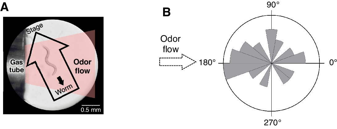
Spatial arrangement of the odor stimulation and behavioral response in the OSB2 system.
(A) Arrangement of the odor flow on the OSB2 system. The end of the tube was positioned ~1 mm from the animal, and odor flow covered the entire body of the animal. Visualization was obtained from the ocular lens of the microscope, and the airflow and direction of an animal's movement and of the stage were overlaid. See also Video 3.(B) Distribution of migratory bearing during negative dC/dt. Bearings of each animal's migratory vector throughout decreases in odor concentration, which were formed by connecting the start and end points of each animals’ trajectory during the odor-down phase, were plotted for the 20 animals that were analyzed in Figure 3B. No significant bias was observed (p>0.1, Watson's U2 test).
Figure 4 with 3 supplements
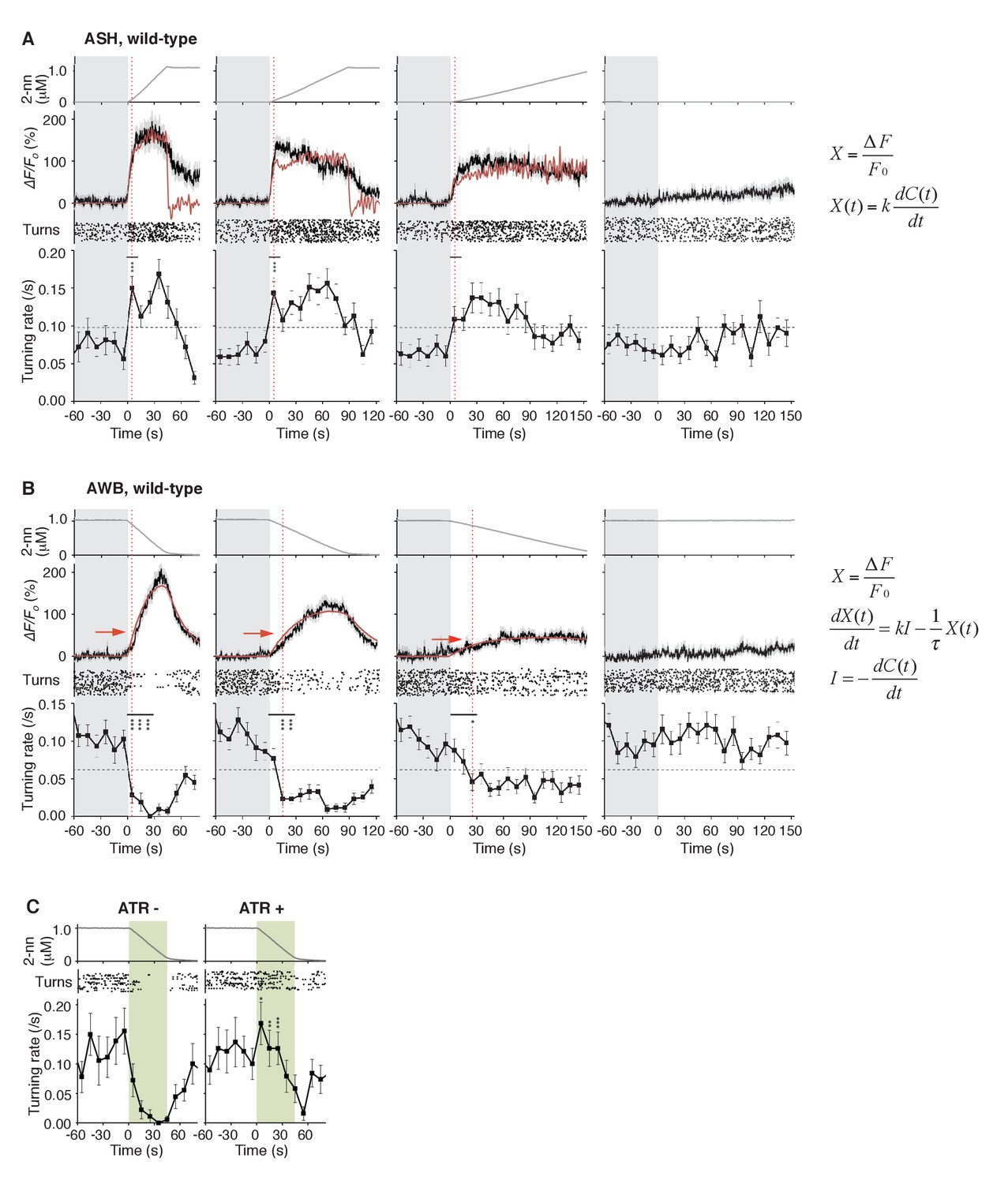
ASH neurons are activated according to dC/dt for initiating turns, and AWB neurons are activated according to the leaky integration of the negative dC/dt for suppressing turns with a dC/dt-dependent delay.
(A) ASH responses (middle panels) and turns (lower panels) in response to odor concentration increases from 0 to 1 μM in 45 s (left most; n = 32), 90 s (middle left; n = 39), 180 s (middle right; n = 35) or no odor increase (‘no odor control’; right most; n = 41) are shown. (Middle panels) In the three conditions with odor increases, the response patterns of ASH neurons (the average ± SEM: black lines and gray shadows, respectively) were fitted by time-differentials of the average of measured odor concentration (red lines), calculated by the rightmost equations. (Lower panels) Ensemble averages of the turning rates ± SEM in each 10 s bin were calculated. The original data is shown in the raster plot. Black horizontal dashed lines in lower panels indicate the upper limit of 99% prediction interval of all the turning rates during the odor-zero phase (t = −60 ~ 0; gray area). Red vertical dotted lines indicate the time when each turning rate first exceeded the upper limit of prediction interval. In the first bin of odor-up phase (indicated by a black horizontal bar in the lower panels), the turning rate in the 45 s and 90 s conditions increased significantly compared to the no-odor control (***p<0.001, Kruskal-Wallis test with post hoc Steel-Dwass test). (B) AWB responses and turns in response to odor concentration decreases from 1 μM (odor-plateau phase; gray area) to 0 μM (odor-zero phase) in 45 s (left-most; n = 42), in 90 s (middle left; n = 43), in 180 s (middle right; n = 48) and no odor decrease (‘odor-plateau control’; right-most; n = 38). AWB responses to different dC/dt rates were fitted by a leaky integrator equation of negative dC/dt (red lines). Black horizontal dashed lines in the lower panels indicate the lower limit of the 99% prediction interval of the turning rates during the odor-plateau phase. The times when the turning rates became lower than the limit (red vertical dotted lines) were delayed when the dC/dt rate was smaller (*p<0.005 and ***p<0.001, Kruskal-Wallis test with post hoc Steel-Dwass test). The statistical test was performed in the first 3 bins of the odor-down phase (a black horizontal bar in lower panels). (C), Effect of optogenetic silencing of the AWB response on negative dC/dt. Transgenic animals expressing Arch in AWB neurons were cultivated in the absence (n = 18) or presence (n = 19) of ATR and illuminated with green light during the odor-down phase. *p<0.05, **p<0.01, and ***p<0.001 (Mann-Whitney test). In the panels, the gray shading means the period with no odor change, in which the prediction intervals were calculated. All the statistical details are shown in Supplementary file 1. The following figure supplements are available for Figure 4.
Figure 4—figure supplement 1

AWB responses were not fitted sufficiently by time-differential equations.
https://doi.org/10.7554/eLife.21629.014
Figure 4—figure supplement 2
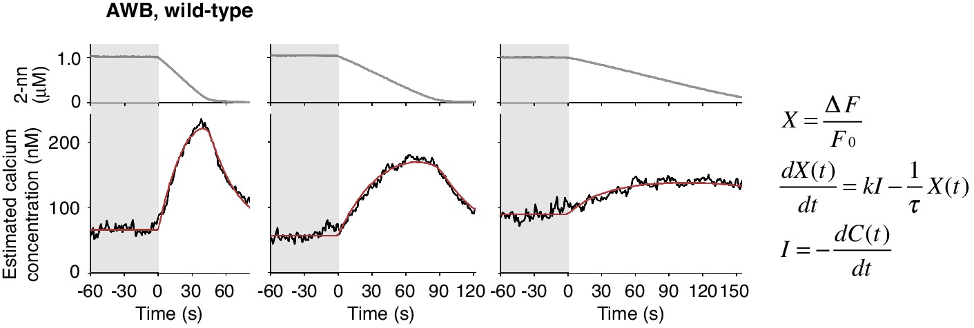
Estimated intracellular calcium concentrations in AWB neurons calculated from measured ΔF/F0 in Figure 4B.
Estimated calcium concentration changes (black lines) in response to odor decreases from 1 to 0 μM in 45 s (left), 90 s (center), and 180 s (right) were also well-fitted by a leaky integrator equation of negative dC/dt (red lines). The calcium affinity (Kd = 405 nM) used for the estimation was according to Akerboom et al. (2012). Other parameters are described in Table 2.
Figure 4—figure supplement 3
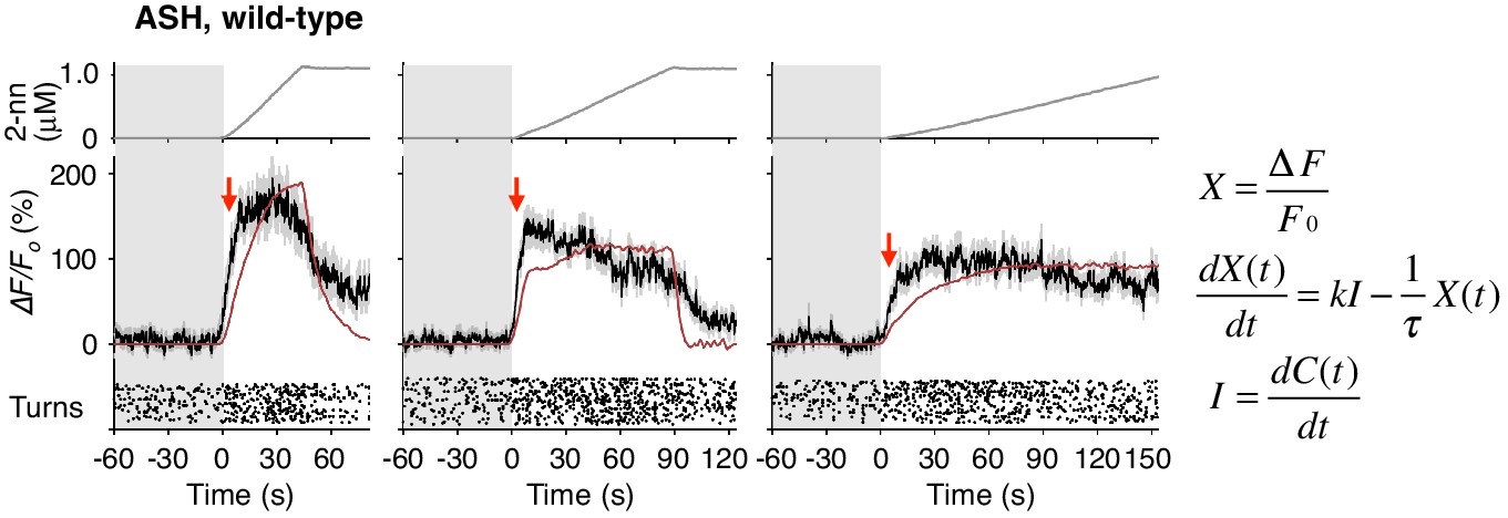
ASH responses were partially fitted by the time-integral equations.
The ASH responses are the same as those in Figure 4A. Red arrows indicate the same timing with the red vertical dotted lines in Figure 4A. The parameters and goodness of fit are described in Table 3.
Figure 5
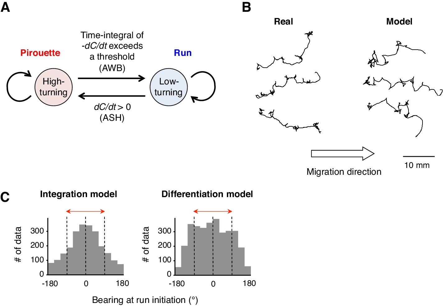
A computer model reproduced the directional choice in the odor avoidance task in a temporal integration-dependent manner.
(A) Model of the behavioral transition in 2-nonanone avoidance. During a pirouette, a model animal frequently repeated turns and short migrations. When a model animal initiated a migration away from the odor source and sensed dC/dt <0, the high-turning state transited to a low-turning state (i.e., a run) when the leaky integrator equation exceeded a threshold. During a run, the animals turned with much lower frequency than in pirouette and at a probability related to dC/dt >0 due to straying away from the original direction. (B) Three typical tracks of real (left) and model (right) animals. As shown in Figure 1A, the odor source is on the left side. (C) Histograms of the initial bearings of runs in the model animals. The high-turning-to-low-turning transition was dependent on temporal integration (left) or on differentiation (right). p<0.001 (Mardia-Watson-Wheeler test). All the statistical details are shown in Supplementary file 1.
Figure 6 with 1 supplement
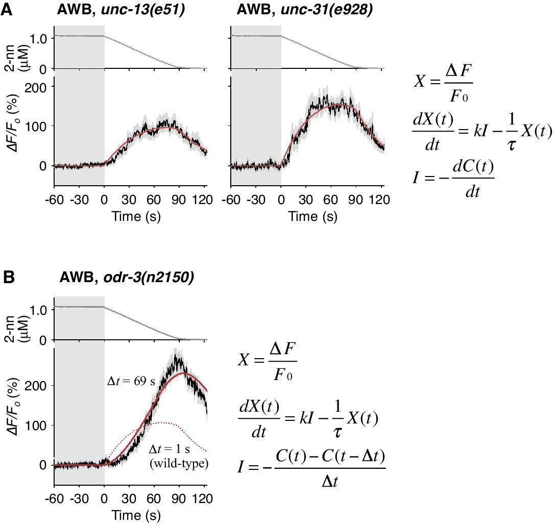
Cell-autonomous computations in AWB neurons.
(A) The AWB responses of unc-13 (left) and unc-31 (right) mutants to the odor decreases, which are the same as those shown in the middle left panel of Figure 4B, were essentially similar to those of wild-type animals and fitted by the leaky integrator equations (n = 31 and 17, respectively). (B) The AWB responses of odr-3(n2150) mutants (n = 24) were fitted by the leaky integrator equation (red solid line) with the time interval (∆t) being much longer than that of wild-type AWB (red dotted line). The parameters are described in Table 2. In the experiments for panels A and B, the behavioral responses were not analyzed because the unc-13, unc-31, and odr-3 mutations affect the activities of multiple neurons, including ASH and AWB.
Figure 6—figure supplement 1
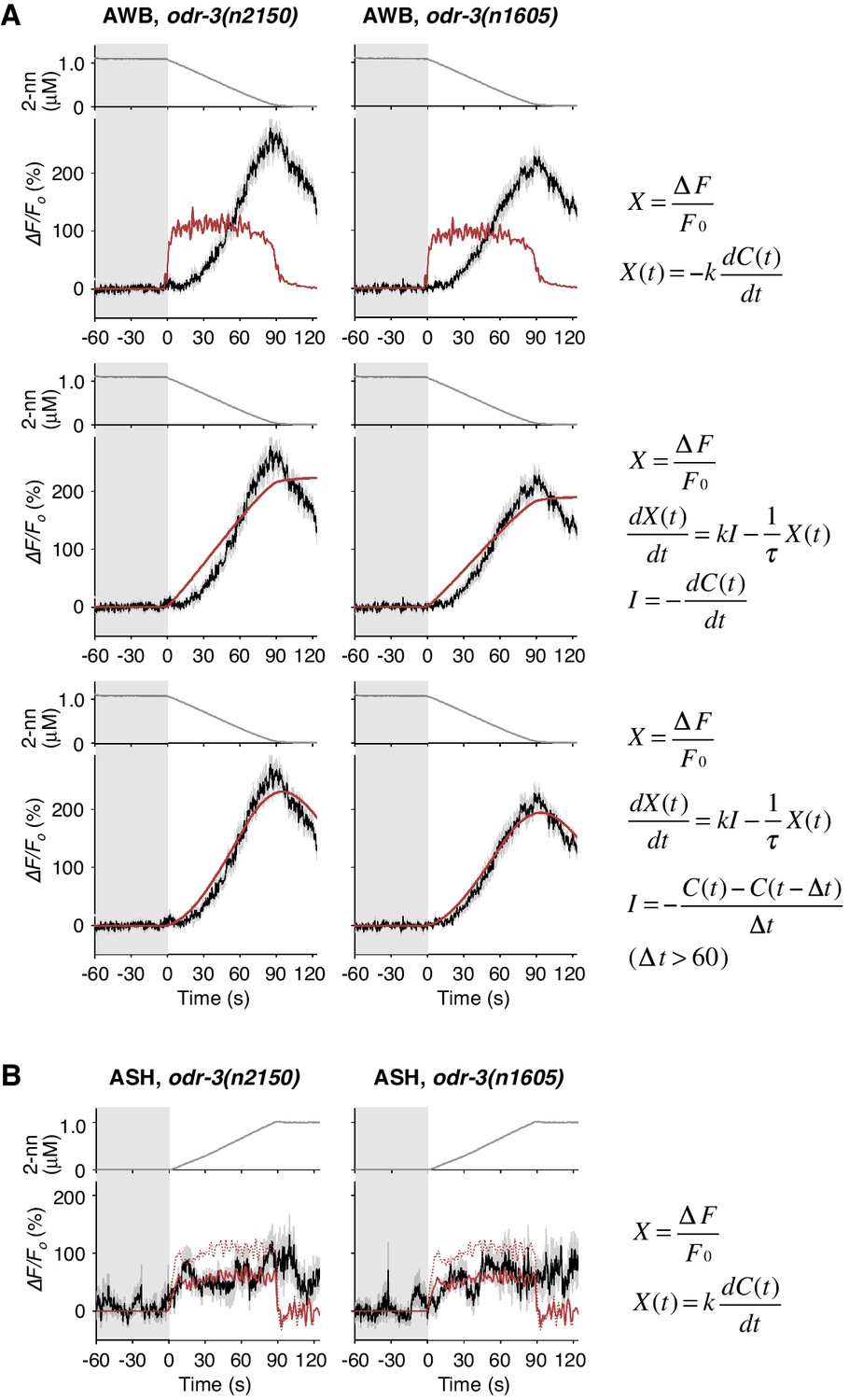
Responses of AWB and ASH neurons in odr-3 mutants.
(A) AWB responses in odr-3(n2150) (left panels; the same data as Figure 6B) or odr-3(n1605) (right panels; n = 28) mutants were fitted by the right-most equations. When fitting with the leaky integrator equation also used in Figure 4B, τ diverged to infinity (middle panels; see Table 4). (B) ASH activity in odr-3(n2150) mutants (left; n = 15) and odr-3(n1605) mutants (right; n = 12) in response to a concentration increase from 0 to 1 μM in 90 s are shown. The ASH activities of odr-3 mutants were also fitted by dC/dt (red solid lines; red dashed lines are the fit to the wild-type response in Figure 4A) although the coefficients k were different from those of wild-type animals (Table 1).
Figure 7 with 1 supplement
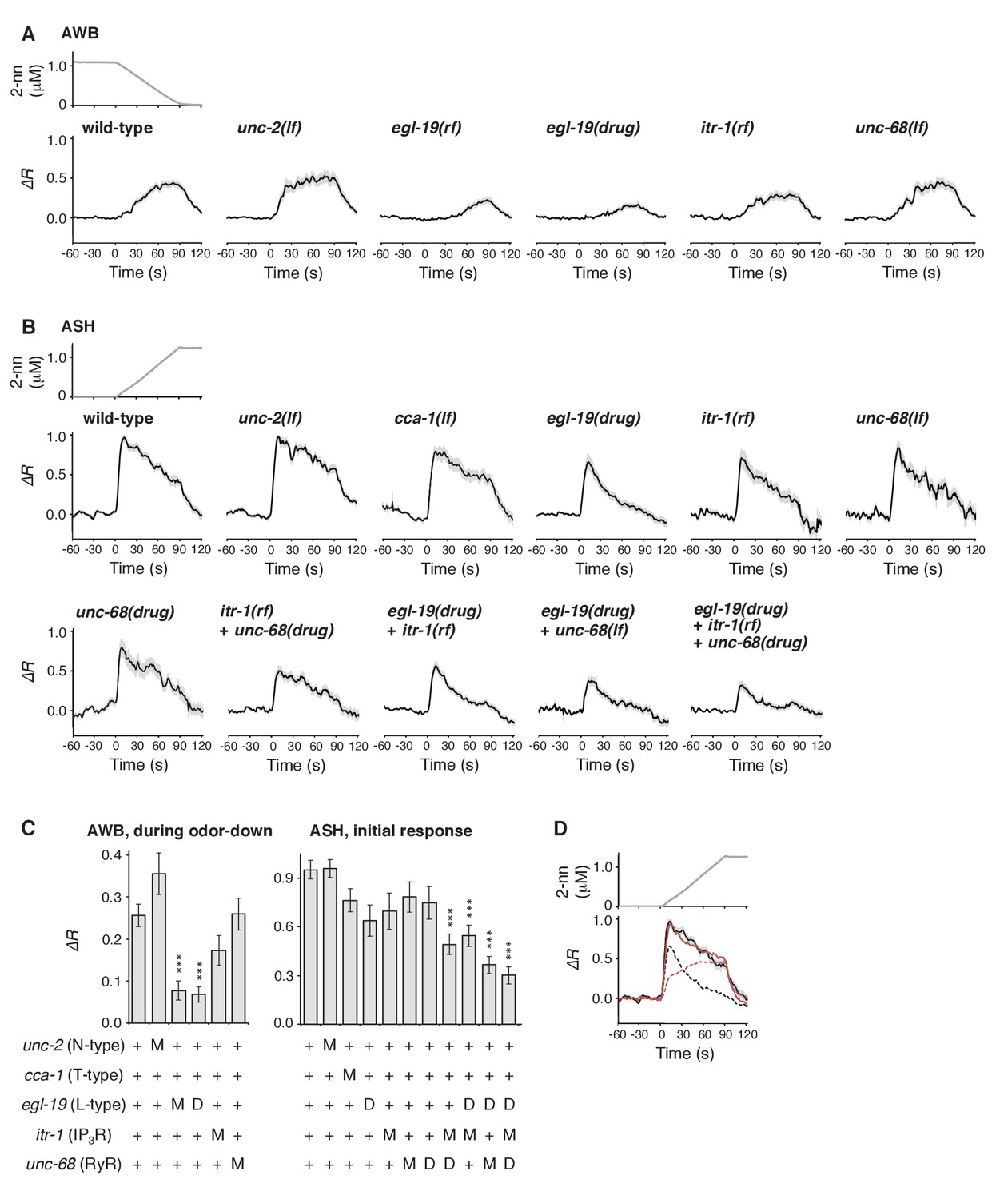
Calcium channels are involved in the dynamic regulation of [Ca2+]i in a cell type-dependent manner.
(A and B) Responses of AWB (panel A) or ASH (panel B) neurons in strains with genetic and/or pharmacological suppression of N/P/Q-type VGCC UNC-2, T-type VGCC CCA-1, L-type VGCC EGL-19, IP3R ITR-1, and RyR UNC-68. lf is a loss-of-function mutation, and rf is a reduction-of-function mutation. Note that loss-of-function mutations of egl-19 and itr-1 are not available due to possible lethality. (C) Suppression of the AWB response during the odor-down phase (left) and of the initial ASH response (10–15 s of the odor-up phase) (right) with the genetic mutation (M) and/or the drug treatment (D). ***p<0.001 (Kruskal-Wallis test with post hoc Steel-Dwass test). (D) egl-19 is also responsible for the slow time-integral component in ASH neurons. Addition of a putative time-integral response using the leaky integrator equation to the transient response in the ‘egl-19(drug)’ reproduced the ASH response of the naive wild-type animals. Black line: wild-type response shown in panel B; black dashed line: egl-19(drug) response in panel B; red dashed line: the time-integral model of positive dC/dt; red line: sum of the black and red dashed lines. The parameters are described in Table 1. All the statistical details are shown in Supplementary file 1.
Figure 7—figure supplement 1
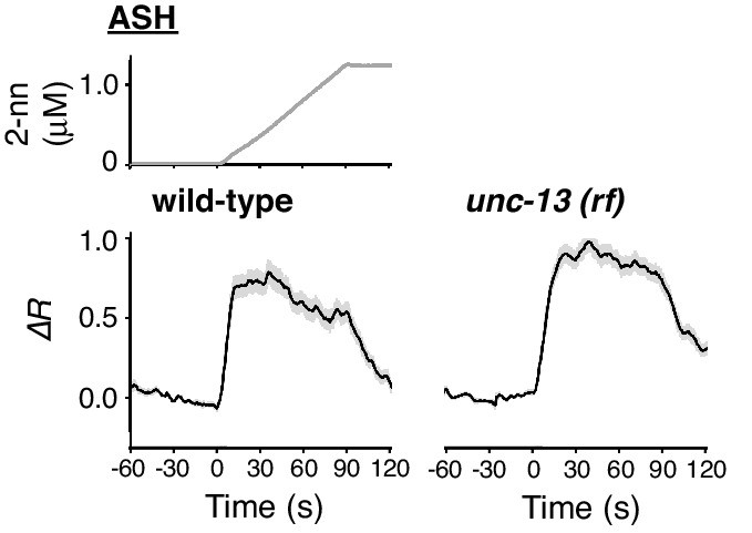
ASH response does not depend on synaptic transmission.
ASH responses in wild-type (left; n = 35) and unc-13(e51) (right; n = 44) animals, analysed in parallel, are shown.
Figure 8
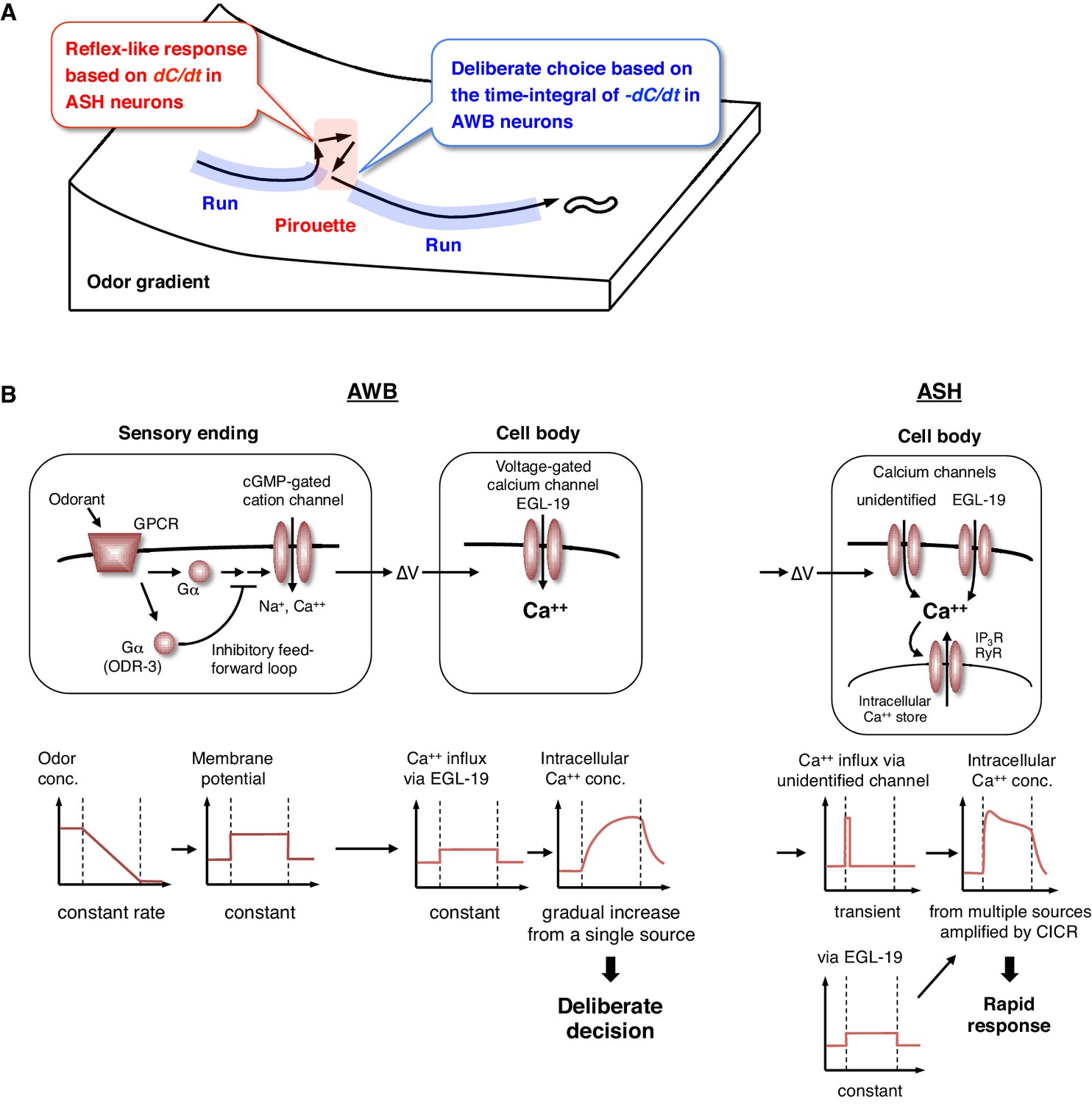
Physiological and molecular models of decision-making by C. elegans during odor avoidance.
(A) Computations of ASH and AWB neurons during odor avoidance behavior. (B) Model of the molecular mechanisms for temporal computation of odor information in AWB and ASH neurons. (Left) In AWB neurons, odor decreases likely cause the activation of Gα proteins as an odor-OFF response (Bargmann, 2006; Usuyama et al., 2012), where an unidentified Gα positively transduces the signal and ODR-3 inhibits the signal for the time-differential computation. The Gα signaling is transmitted to the cGMP-gated cation channel TAX-2/TAX-4 (Bargmann, 2006) to cause depolarization. Depolarization then triggers calcium influx via EGL-19 at the cell body, which causes the gradual accumulation of [Ca2+]i. (Right) In ASH neurons, the depolarization at the sensory ending triggers an unidentified rapid and transient calcium channels, as well as EGL-19. The calcium influx through these channels is amplified by CICR via RyR (UNC-68) and IP3R (ITR-1).
Videos
Video 1
Time-course changes in the fitted 2-nonanone concentration.
Although the odor sources were two circles of ~5 mm diameter in the real experiment, they were treated as points in the simulation.
Video 2
A demonstration video for calcium imaging with the OSB2 system.
(Left) The bright field images for the tracking and the fluorescence images for calcium imaging were acquired simultaneously but separately in the tracking and calcium imaging subsystems, respectively. The video was compiled separately because of the different frame rates and ran on a Power Point file. Because of a technical limitation on the video playing, the videos were not completely synchronized. (Right) From the fluorescence images, the cell body of AWB neuron was tracked and centered off-line. The video speed is 2.8x.
Video 3
Visualization of the odor flow on the OSB2 system.
The view was from the ocular lens of the microscope. The tube end was on the left and the flow was from the left to the right, which was visualized by fog produced by Wizard Stick (Zero Toys, USA). Contrast of the video image was enhanced for visualization of the flow. The worm was immobilized for reference. The video speed is 1x.
Video 4
Optogenetic activation of AWB neurons.
After 60 s without any stimulus, a transgenic animal expressing the bistable variant of channelrhodopsin, ChR2(C128S), was illuminated with blue light for 3 s to cause sustained AWB activation, and the behavior was monitored for the following 30 s. The video speed is 8x.
Tables
Table 1
Models and parameters used in the fitting of ASH responses with time-differential equations.
| Conditions | ASH, wild-type | ASH, odr-3(n2150) | ASH, odr-3(n1605) | ASH, wild-type slow component | ||
|---|---|---|---|---|---|---|
| Durations of up/down phase | Up 45 s | Up 90 s | Up 180 s | Up 90 s | Up 90 s | Up 90 s |
| Model | ||||||
| Parameters used for fitting to ΔF/F0 | ||||||
| k | 56.1 [μM−1·s] | 80.9 [μM−1·s] | 121.9 [μM−1·s] | 49.1 [μM−1·s] | 46.7 [μM−1·s] | 2.96 [μM−1] |
| τ | - | - | - | - | - | 10.4 [s] |
| Parameters used for fitting to estimated calcium concentration | ||||||
| k | 3.9 [s] | 6.2 [s] | 7.9 [s] | 2.8 [s] | 2.9 [s] | - |
| τ | - | - | - | - | - | - |
| fmax | 9.4 | 9.5 | 9.2 | 9.1 | 8.7 | - |
| fmin | 0.79 | 0.79 | 0.77 | 0.76 | 0.73 | - |
| Xbase | 103.8 [nM] | 92.2 [nM] | 107.0 [nM] | 108.2 [nM] | 109.7 [nM] | - |
Table 2
Models and parameters used in the fitting of AWB responses with leaky integrator equations.
| Conditions | AWB, wild-type | AWB, unc-13(e51) | AWB, unc-31(e928) | AWB, odr-3(n2150) | AWB, odr-3(n1605) | ||
|---|---|---|---|---|---|---|---|
| Durations of up/down phase | Down 45 s | Down 90 s | Down 180 s | Down 90 s | Down 90 s | Down 90 s | Down 90 s |
| Model | |||||||
| (∆t = 67 s) | (∆t = 66 s) | ||||||
| Parameters used for fitting to ΔF/F0 | |||||||
| k | 4.6 [μM−1] | 3.6 [μM−1] | 3.0 [μM−1] | 2.6 [μM−1] | 4.9 [μM−1] | 8.7 [μM−1] | 7.7 [μM−1] |
| τ | 19.7 [s] | 28.1 [s] | 25.0 [s] | 34.5 [s] | 28.1 [s] | 25.2 [s] | 23.5 [s] |
| Parameters used for fitting to estimated calcium concentration | |||||||
| k | 0.40 | 0.37 | 0.33 | 0.26 | 0.44 | 1.00 | 0.87 |
| τ | 21.1 [s] | 28.5 [s] | 25.0 [s] | 37.3 [s] | 30.7 [s] | 17.7 [s] | 17.7 [s] |
| fmax | 9.7 | 10.1 | 8.5 | 9.6 | 8.9 | 10.9 | 10.4 |
| fmin | 0.81 | 0.84 | 0.71 | 0.80 | 0.74 | 0.91 | 0.87 |
| Xbase | 66.1 [nM] | 56.7 [nM] | 89.6 [nM] | 66.7 [nM] | 81.2 [nM] | 41.8 [nM] | 51.5 [nM] |
Table 3
Parameters and goodness of fit results for mathematical models of ASH and AWB responses.
| Conditions | ASH, wild-type | AWB, wild-type | ||||
|---|---|---|---|---|---|---|
| Durations of up/down phase | Up 45 s | Up 90 s | Up 180 s | Down 45 s | Down 90 s | Down 180 s |
| Number of samples (frames) used for calculation of BIC | N = 135 (t = −60 ~ 75 s) | N = 180 (t = −60 ~ 120 s) | N = 270 (t = −60 ~ 210 s) | N = 135 (t = −60 ~ 75 s) | N = 180 (t = −60 ~ 120 s) | N = 270 (t = −60 ~ 210 s) |
| k = 56.1 [μM−1·s] BIC = −222.2 | k = 80.9 [μM−1·s] BIC = −446.5 | k = 121.9 [μM−1·s] BIC = −637.8 | k = −58.4 [μM−1·s] BIC = −170.6 | k = −73.4 [μM−1·s] BIC = −372.5 | k = −67.3 [μM−1·s] BIC = −1157 | |
| k = 5.8 [μM−1] τ = 12.0 [s] BIC = −331.1 | k = 18.9 [μM−1] τ = 4.4 [s] BIC = −472.8 | k = 11.5 [μM−1] τ = 11.7 [s] BIC = −804.9 | k = −4.56 [μM−1] τ = 19.7 [s] BIC = −591.9 | k = −3.58 [μM−1] τ = 28.1 [s] BIC = −806.2 | k = −3.01 [μM−1] τ = 25.0 [s] BIC = −1458 | |
Table 4
Parameters and goodness of fit for mathematical models of AWB responses in odr-3 mutants.
| Conditions | AWB, odr-3(n2150) | AWB, odr-3(n1605) |
|---|---|---|
| Durations of up/down phase | down 90 s | down 90 s |
| Number of samples (frames) used for calculation of BIC | N = 180 (t = −60 ~ 120 s) | N = 180 (t = −60 ~ 120 s) |
| k = 89.1 [μM−1·s] BIC = 25.1 | k = 77.3 [μM−1·s] BIC = −39.2 | |
| k = 2.08 [μM−1] τ → ∞ BIC = −477.7 | k = 1.77 [μM−1] τ → ∞ BIC = −578.5 | |
| k = 8.71 [μM−1] τ = 25.2 [s] ∆t = 67 [s] BIC = −645.6 | k = 7.73 [μM−1] τ = 23.5 [s] ∆t = 66 [s] BIC = −779.9 |
Additional files
-
Supplementary file 1
Detailed results of statistical tests in this study are shown.
- https://doi.org/10.7554/eLife.21629.027
-
Supplementary file 2
Plasmids used in this study are shown.
- https://doi.org/10.7554/eLife.21629.028
-
Supplementary file 3
Strains used in this study are shown.
- https://doi.org/10.7554/eLife.21629.029
Download links
A two-part list of links to download the article, or parts of the article, in various formats.
Downloads (link to download the article as PDF)
Open citations (links to open the citations from this article in various online reference manager services)
Cite this article (links to download the citations from this article in formats compatible with various reference manager tools)
Calcium dynamics regulating the timing of decision-making in C. elegans
eLife 6:e21629.
https://doi.org/10.7554/eLife.21629


