Neural markers of predictive coding under perceptual uncertainty revealed with Hierarchical Frequency Tagging
- Philosophy Department, Monash University, Australia
- The University of New South Wales, Australia
- Monash University, Australia
Figures
Figure 1
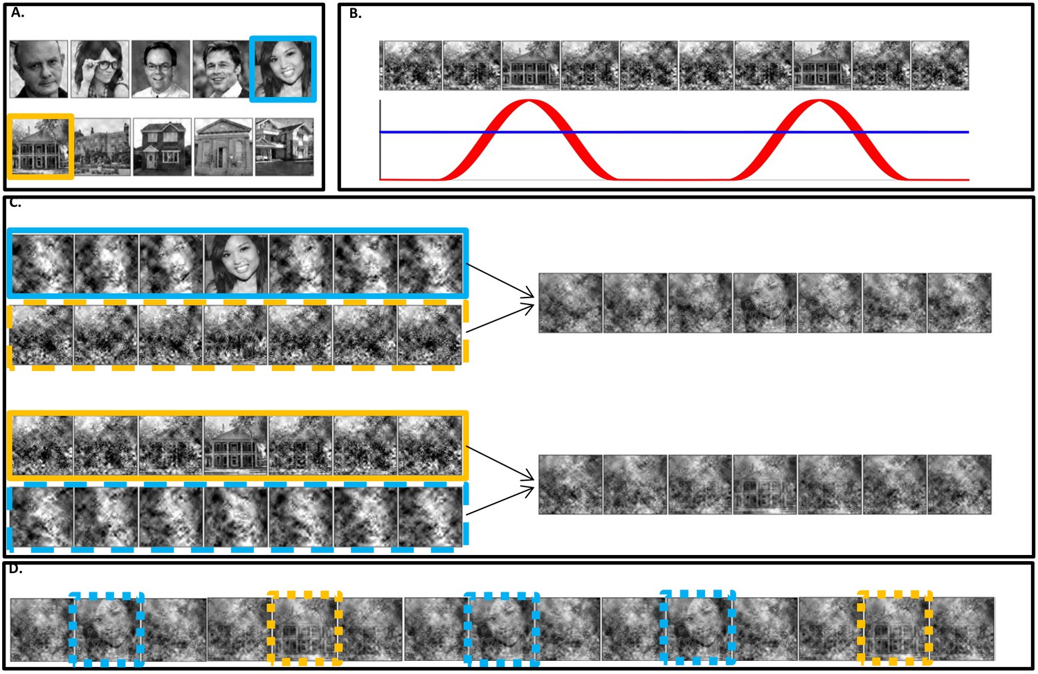
Stimuli construction.
Schematic illustration of stimuli construction. (A) A pool of 28 face and 28 house images were used in the paradigm (images with ‘free to use, share or modify, even commercially’ usage rights, obtained from Google Images). (B) The SWIFT principle. Cyclic local-contour scrambling in the wavelet-domain allows us to modulate the semantics of the image at a given frequency (i.e. the tagging-frequency, F2 = 1.3 hz, illustrated by the red line) while keeping low-level principal physical attributes constant over time (illustrated by the blue line) (C) Each trial (50 s) was constructed using one SWIFT cycle (~769 ms) of a randomly chosen face image (blue solid rectangle) and one SWIFT cycle of a randomly chosen house image (orange solid rectangle). For each SWIFT cycle, a corresponding ‘noise’ SWIFT cycle was created based on one of the scrambled frames of the original SWIFT cycle (orange and blue dashed rectangles). Superimposition of the original (solid rectangles) and noise (dashed rectangles) SWIFT cycles ensures similar principal local physical properties across all SWIFT frames, regardless of the image appearing in each cycle. (D) The two SWIFT cycles (house and face) were presented repeatedly in a pseudo-random order for a total of 65 cycles. The resulting trial was a 50 s movie in which images peaked in a cyclic manner (F2 = 1.3 Hz). Finally, a global sinusoidal contrast modulation at F1 = 10 Hz was applied onto the whole movie to evoke the SSVEP.
Figure 2

Amplitude SNR spectra.
Amplitude SNRs (see Materials and methods for the definition of SNR), averaged across all electrodes, trials and participants, are shown for frequencies up to 23 Hz. Peaks can be seen at the tagging frequencies, their harmonics and at IM components. Solid red lines mark the SSVEP frequency and its harmonic (10 Hz and 20 Hz, both with SNRs significantly greater than one). Solid pink lines mark the SWIFT frequency and harmonics with SNRs significantly greater than one (n2f2 where n2 = 1,2,3…8 and 11). Solid black lines mark SWIFT harmonics with SNRs not significantly greater than one. Yellow dashed lines mark IM components with SNRs significantly greater than one (n1f1 + n2f2; n1 = 1, n2 = +−1,+−2,+−3,+−4 as well as n1 = 2, n2 = −1,+2) and black dashed lines mark IM components with SNRs not significantly greater than one.
Figure 3 with 1 supplement
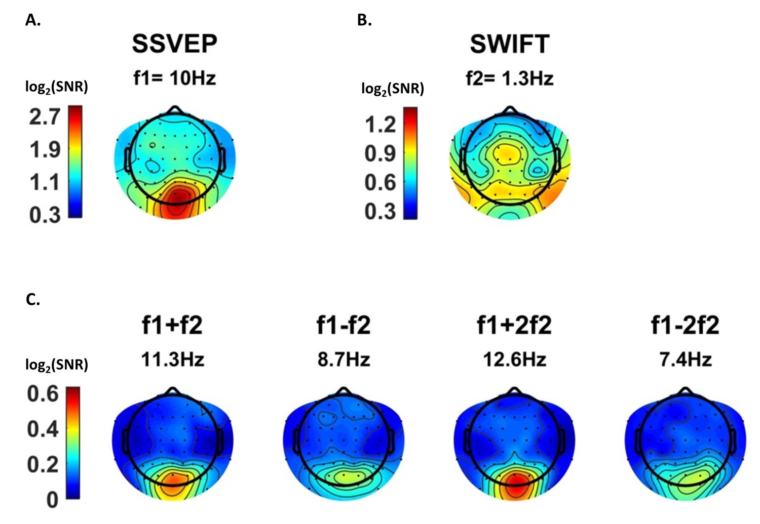
Scalp distributions.
Topography maps (log2(SNR)) for SSVEP (f1 = 10 Hz) (A), SWIFT (f2 = 1.3 Hz) (B), and four IM components (f1+f2, f1−f2, f1+2f2 and f1−2f1) (C). SSVEP SNRs were generally stronger than SWIFT SNRs, which in turn were stronger than the IM SNRs (note the different colorbar scales).
Figure 3—figure supplement 1

As a measure of the similarity between the scalp distributions of the SSVEP, SWIFT and IM frequencies, we examined the Pearson correlation between the mean SNR values across participants for the IM, SSVEP and SWIFT frequencies across all 64 channels (each point represents the mean SNR for a single channel across 17 participants).
To examine whether the correlation coefficients for the comparison between the IMs and the SSVEP were higher than the correlation coefficients for the comparison between the IMs and the SWIFT, we applied the Fisher’s r to z transformation and performed a Z-test for the difference between correlations. We found that the distributions of all IM components were more highly correlated with the SSVEP than with the SWIFT distribution (z = 6.44, z = 5.52, z = 6.5 and z = 6.03 for f1 +f2, f1-f2, f1 +2f2 and f1-2f2, respectively; two-tailed, FDR adjusted p<0.01 for all comparisons).
Figure 4
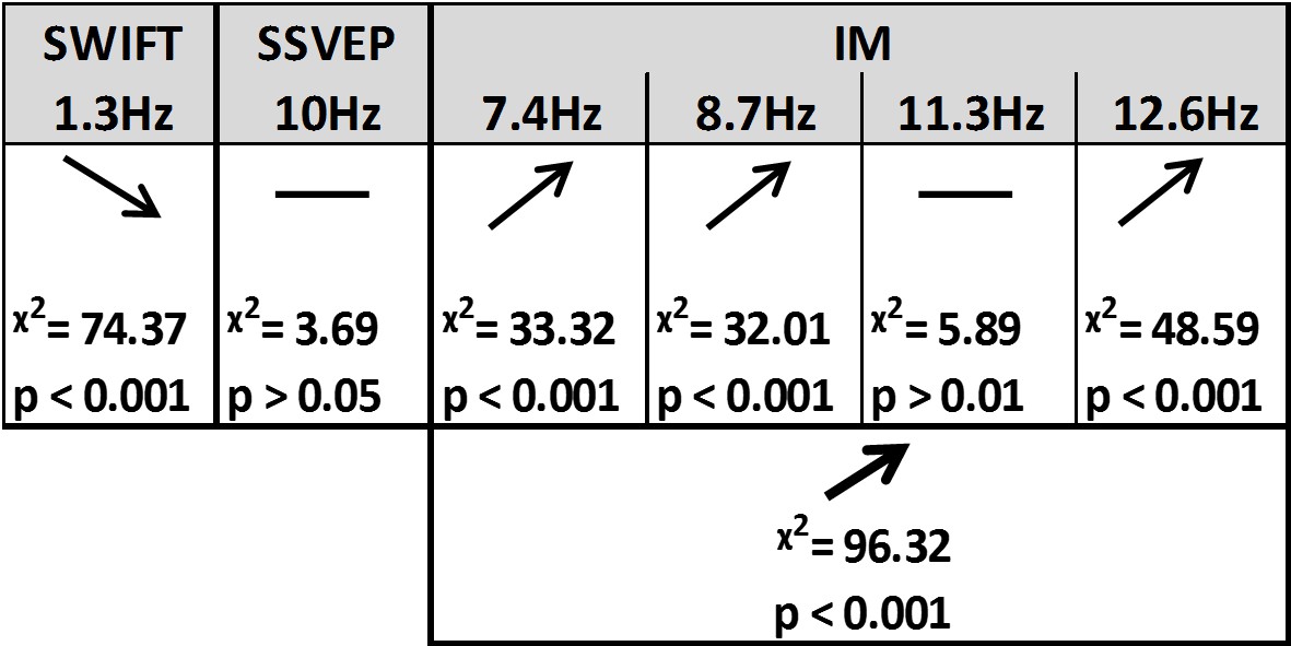
Summary of the linear mixed-effects (LME) modelling.
We used LME to examine the significance of the effect of certainty for SSVEP (f1 = 10 Hz), SWIFT (f2 = 1.3 Hz) and IM (separately for f1−2f2, f1−f2, f1+f2, and f1+2f2, as well as across all four components) recorded from posterior ROI electrodes. The table lists the direction of the effects, χ2 value and FDR-corrected p-value from the likelihood ratio tests (See Materials and methods).
Figure 5
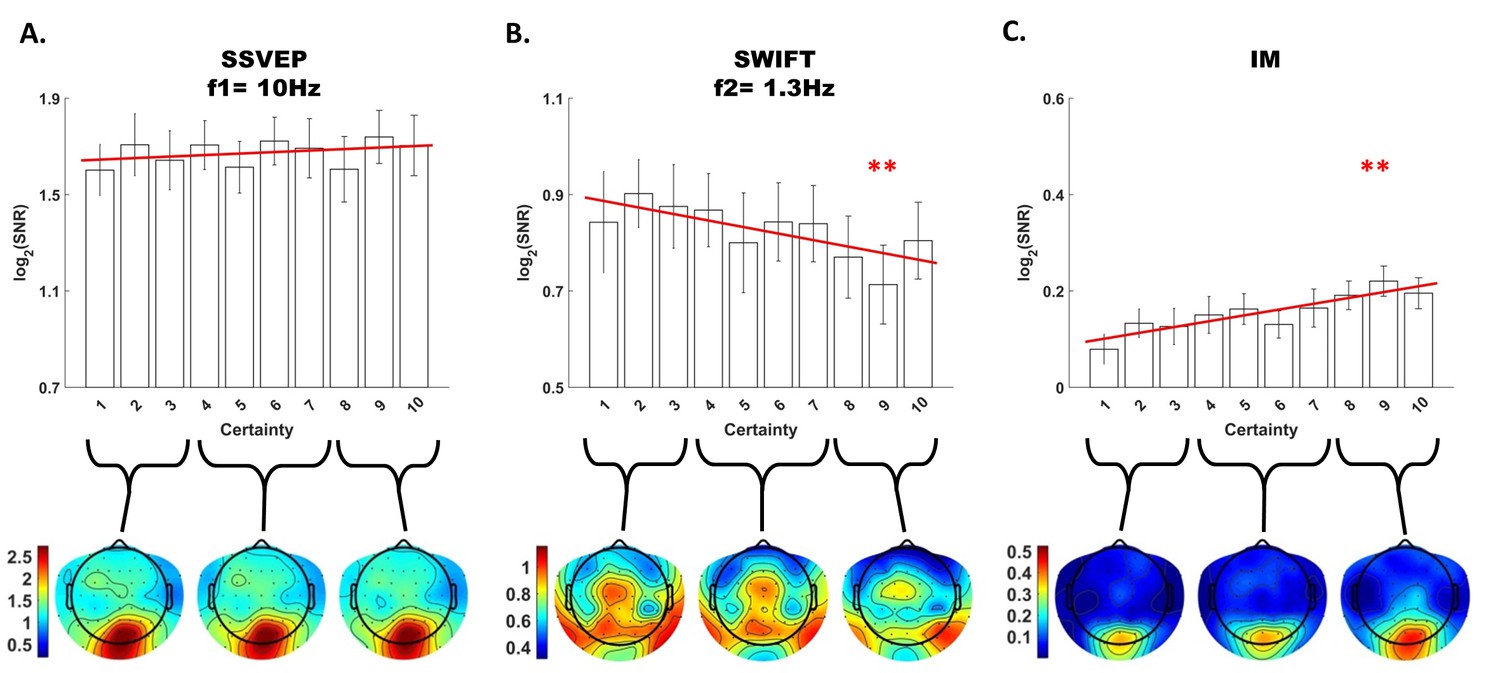
Modulation by certainty.
Bar plots of signal strength (log of SNR, averaged across 30 posterior channels and 17 participants) as a function of certainty levels for SSVEP (A), SWIFT (B) and IMs (averaged across the 4 IM components) (C). Red lines show the linear regressions for each frequency category. Slopes that are significantly different from 0 are marked with red asterisks (** for p<0.001). While no significant main effect of certainty was found for the SSVEP (p>0.05), a significant negative slope was found for the SWIFT, and a significant positive slope was found for the IM. Error bars are SEM across participants. Bottom) Topo-plots, averaged across participants, for low certainty (averaged across bins 1–3), medium certainty (averaged across bins 4–7) and high certainty (averaged across bins 8–10) are shown for SSVEP (A), SWIFT (B) and IM (averaged across the 4 IM components) (C).
Figure 6
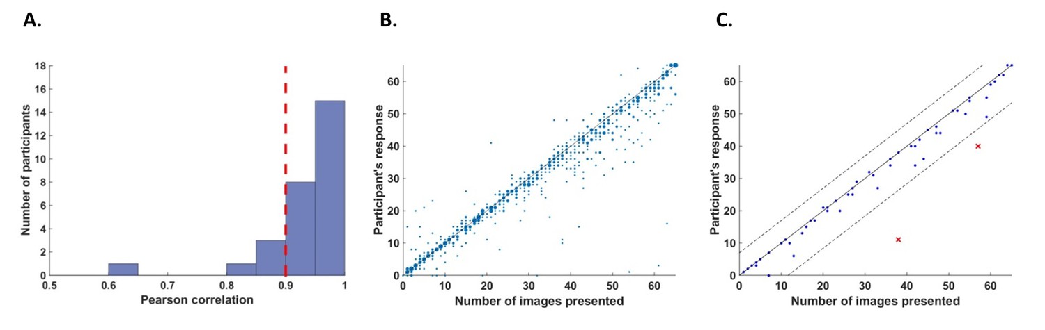
Behavioral performance.
(A) Histogram across all participants for counting accuracy measured as the correlation between the participant’s response (number of image presentations counted in each trial) and the actual number of presentations. Five participants with a counting accuracy below r = 0.9 (vertical red dashed line) were excluded from the analysis. (B) Scatter plot showing responses across 56 trials for all participants included in the analysis. The size of each dot corresponds to the number of occurrences at that point. (C) An example scatter plot for a single participant demonstrating the within-participant exclusion criterion for single trials. The solid line (y=x) illustrates the theoretical location of accurate responses. For each trial, we calculated the distance between the participant’s response and the actual number of cycles in which the relevant image was presented (i.e., the distance between each dot in the plot and the solid line). The within-participant cutoff was then defined as ±2.5 standard deviations from the mean of this distance. Dashed lines mark the within-participant cutoff for exclusion of single trials.
Videos
Video 1
A slow-motion representation of two SWIFT cycles.
https://doi.org/10.7554/eLife.22749.008
Video 2
An 8 s animated movie representation of a HFT trial.
https://doi.org/10.7554/eLife.22749.009
Video 3
A slow motion animation of the first few cycles within a HFT trial.
https://doi.org/10.7554/eLife.22749.010Download links
A two-part list of links to download the article, or parts of the article, in various formats.
Downloads (link to download the article as PDF)
Open citations (links to open the citations from this article in various online reference manager services)
Cite this article (links to download the citations from this article in formats compatible with various reference manager tools)
Neural markers of predictive coding under perceptual uncertainty revealed with Hierarchical Frequency Tagging
eLife 6:e22749.
https://doi.org/10.7554/eLife.22749


