Computational models of O-LM cells are recruited by low or high theta frequency inputs depending on h-channel distributions
- Krembil Research Institute, University Health Network, Canada
- University of Toronto, Canada
Figures
Figure 1 with 3 supplements
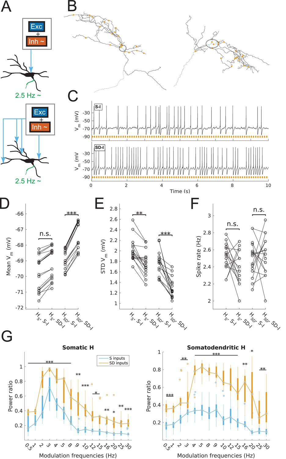
Spiking output of O-LM cell models with somatic or somatodendritic artificial synaptic inputs.
(A) Schematic of the virtual protocol for somatic (top) and somatodendritic (bottom) synaptic inputs. Representative O-LM model morphology shown with soma and dendrites (black) and truncated axon (green). Excitatory and inhibitory Poisson process synaptic inputs shown in grey box; note that each synaptic input location has an independent excitatory and inhibitory Poisson process. Synaptic inputs are tuned to produce approximately 2.5 Hz output prior to input modulation. Only the inhibitory inputs are modulated (‘~' symbol). See Materials and methods for full details. (B) Locations of synaptic inputs when distributed along soma and dendrites (SD inputs case; see Materials and methods) for both O-LM cell morphologies (cell 1, left; cell 2, right; dendrites in black; soma in blue with surrounding dashed black ellipse; truncated axon in grey; synaptic input locations in orange). The case with somatic inputs contains only one input location at the middle of the soma (not shown). (C) Example somatic voltage traces from a model with somatodendritic H (HSD, rank 109) showing spike trains with 8 Hz modulation for somatic inputs (S-I, top) and somatodendritic inputs (SD-I, bottom). Orange bars at bottom denote peak phase of modulation at 8 Hz (see Materials and methods). (D) Mean subthreshold Vm for models with somatic (HS) vs. somatodendritic (HSD) H distributions and somatic inputs (S-I) vs. somatodendritic (SD-I) inputs, all with no modulation (HS: no significant difference, n = 16; HSD: ***p<0.001, n = 16; Wilcoxon rank sum test performed for both cases). (E) Fluctuations of subthreshold Vm of models with HS vs. HSD and S-I vs. SD-I, all with no modulation, as measured by the standard deviation of subthreshold Vm. (HS: **p<0.01, n = 16, Wilcoxon rank sum test; HSD: ***p<0.001, n = 16, paired t-test). (F) Spike rates of models with HS vs. HSD and S-I vs. SD-I, all with no modulation, with no significant difference for both HS and HSD cases (n.s., n = 16 each; paired t-test performed for both). (G) Power ratio, or ratio of power at modulation frequency to 0 Hz frequency, for models with HS (somatic H, left) and HSD (somatodendritic H, right), with S-I (blue) and SD-I (orange). Power ratios are significantly higher for all modulation frequencies for both HS and HSD models. Statistical tests used were two-way repeated measures ANOVA performed separately on the populations of HS and HSD models, between all modulation frequencies crossed with input location (HS: F(1,15) = 13.55, p<0.001, n = 16; HSD: F(1,15) = 5.027, p=0.017, n = 16; Huynd-Feldt correction reported for both tests). Boxplots denote median of power ratios at the circle; 25th and 75th percentiles are denoted by the extent of the thick coloured bars; full extent of data denoted by thin lines extending from the bars, with outliers shown as coloured open circles. Outliers are defined as points outside of q3 ± 2.7σ(q3 – q1), where q1 and q3 are the 25th and 75th percentiles, respectively (see boxplot function in MATLAB). Stars denote level of significance from Tukey’s post-hoc tests, with p<0.05 (*), p<0.01 (**), and p<0.001 (***). Multiple modulation frequencies sharing the same level of significance are connected with a horizontal bar above. When there are no stars at a particular modulation frequency, this denotes no statistical difference was found between the two populations. If no statistical difference was found across all frequencies, a horizontal bar across all x-axis values is placed with a label of ‘n.s.’ on top, meaning ‘not significant’. All subsequent boxplots in later figures share this design.
Figure 1—figure supplement 1
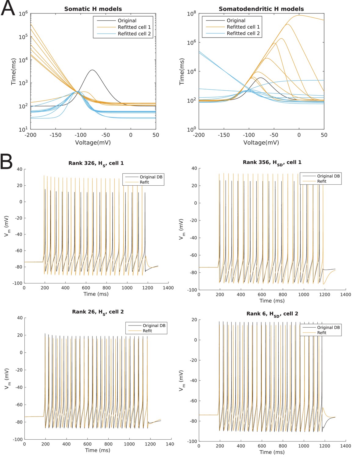
Model spiking responses before and after optimizing passive properties and h-channel kinetics.
(A) Curves for time constant of activation of Ih before (‘Original’) and after optimization. One curve shown per model, with different colours for H distributions. (B) Sample output traces of one of each morphology and dendritic H distribution, using the time constant of activation of Ih, specific membrane resistivity (Rm), and specific membrane capacitance (Cm) from the original database from Sekulić et al. (2014) (black) as well as optimized values for these parameters used in the current work (orange).
Figure 1—figure supplement 2
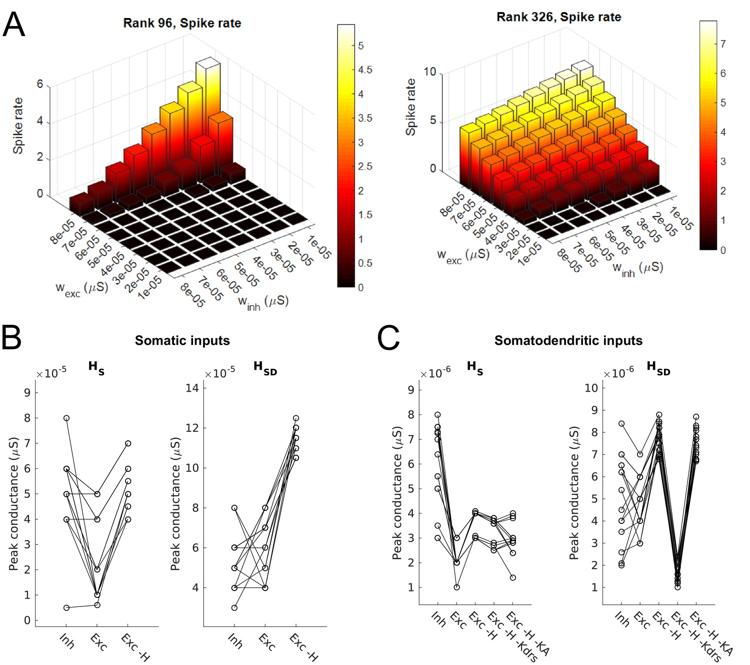
Synaptic parameters for models.
(A) Sample range of varied values for inhibitory and excitatory synaptic conductances (x,y-axes) for an example model with somatic H and morphology 1 (left) and somatodendritic H and morphology 2 (right), resulting in differences in firing rates (z-axis). Heat map corresponds to firing frequency (Hz). (B,C) Excitatory and inhibitory peak synaptic conductances used for each model under various conditions with either somatic (B) or somatodendritic (C) synaptic inputs. Lines connect models that share synaptic parameters under various conditions. All conditions with varying excitatory ‘Exc’ peak conductances share the same inhibitory peak conductance (‘Inh’). Somatic H (HS) and somatodendritic H (HSD) models shown separately for each synaptic input location case. Simulations with various conductances blocked are indicated as follows: ‘-H’ for H block; ‘-H -Kdrs’ for H and Kdrs block; ‘-H -KA’ for H and KA block. The peak excitatory conductances reported for all of these cases with blocked channels refer to the adjusted excitatory synaptic peak conductance to maintain approximately 2.5 Hz baseline firing; see Materials and methods.
Figure 1—figure supplement 3
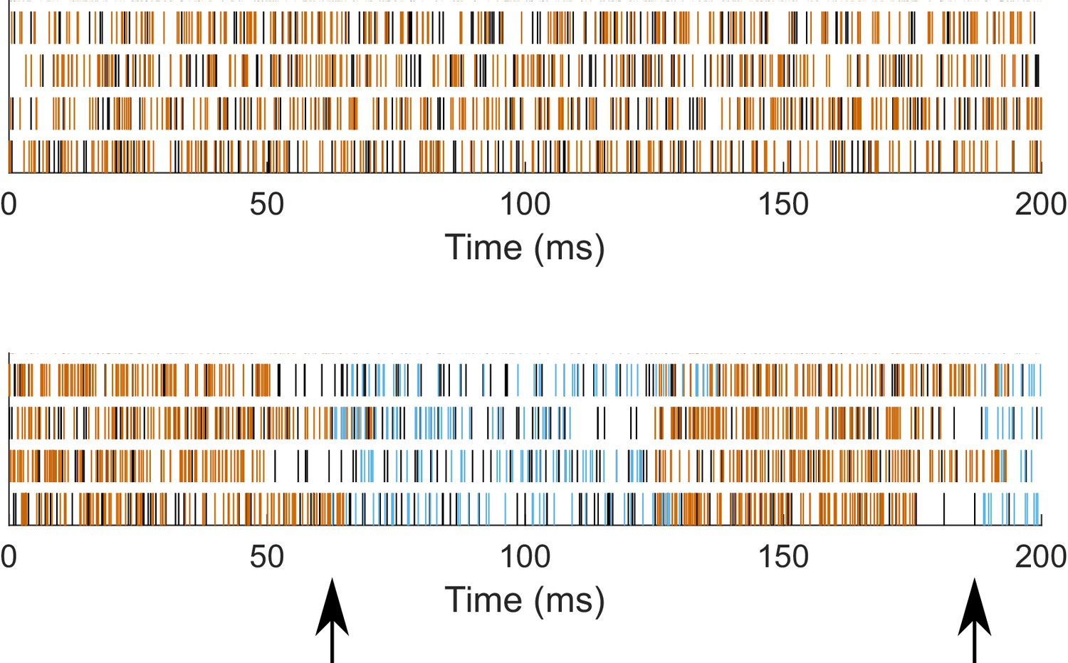
Patterning of synaptic inputs.
Synaptic event times for Poisson trains of unmodulated (top) and modulated (bottom, 8 Hz) synaptic inputs for four locations in the case of somatodendritic inputs, for a sample model with somatodendritic H (model rank 26). Black - excitatory events; Orange - inhibitory events in unmodulated (top) and ‘peak’ of inhibition in modulated (bottom); Blue - inhibitory events during ‘trough’ of inhibition in modulated (bottom). Arrows (bottom) denote time of change from peak to trough periods, that is, the release from peak inhibition.
Figure 2 with 2 supplements
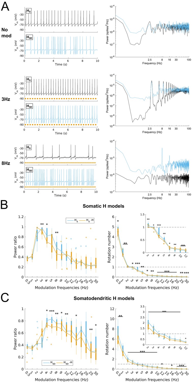
Effects of dendritic H distribution and H block on recruitment of O-LM model spiking in response to modulated somatodendritic inhibitory input.
(A) Somatic Vm traces for example somatic H model (HS, black) and somatodendritic H model (HSD, blue) under various modulation conditions (top – no modulation; middle – 3 Hz modulation; bottom – 8 Hz modulation). With modulated inputs, orange bars at bottom denote phase of peak modulation at the specified frequency (see Materials and methods). Power spectrum density (PSD) plots shown to the right of each output trace. (B, C) Power ratios (left) and rotation numbers (right) under different modulation frequencies for models with somatic H (B) and somatodendritic H (C) in control and H blocked (‘-H’) conditions. Insets in rotation number plots show zoomed portion in the theta range (2–12 Hz). Statistical test used was repeated measures ANOVA for the populations of HS and HSD models between all modulation frequencies crossed with H block condition (power ratios HS: F(1,15) = 2.23, p=0.013, n = 16; HSD: F(1,15) = 2.89, p=0.017, n = 16; rotation numbers HS: F(1,15) = 27.94, p<0.001, n = 16; HSD: F(1,15) = 10.35, p=0.006, n = 16; Huynd-Feldt correction reported for all tests). Boxplot annotations as per Figure 1G legend.
Figure 2—figure supplement 1
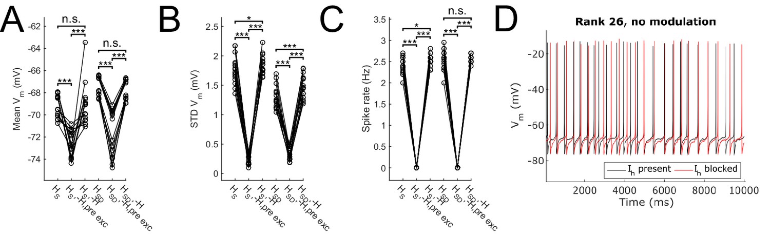
Effect of blocking H on sub- and suprathreshold measures.
Somatic Vm means (A), fluctuations, expressed as standard deviation (B), and firing rates (C) without modulation and in control, H block (‘-H, pre exc’), and adjusting for H block by increased excitatory peak conductance (‘-H’). (D) Somatic Vm trace of a sample model in control (black) as well as H block with increased excitatory conductance (red). Statistical test throughout was 2-sample t-test, with p<0.05 (*), p<0.001 (***), and n.s. denoting not significant. n = 16 for each HS and HSD population.
Figure 2—figure supplement 2
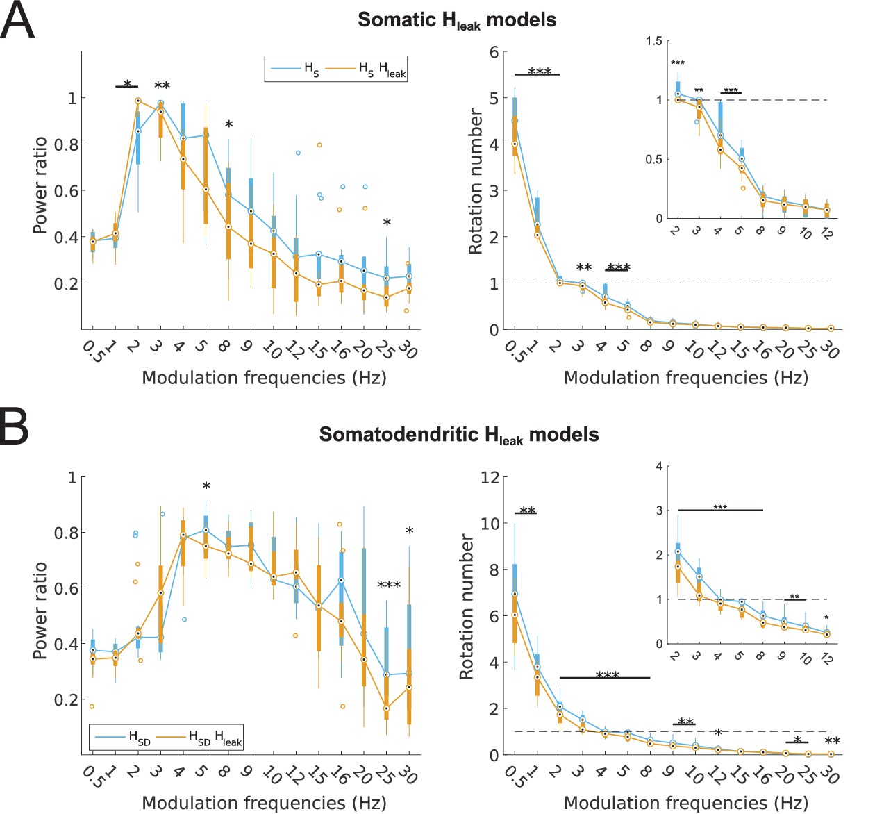
Partitioning of spiking responses of O-LM models into high and low theta when using ‘H leak’ instead of H block.
(A, B) Power ratios (left) and rotation numbers (right) under different modulation frequencies for models with somatic H (A) and somatodendritic H (B) in control and H leak (‘H leak’) conditions. Insets in rotation number plots show zoomed portion in the theta range (2–12 Hz). Statistical test used was repeated measures ANOVA for the populations of HS and HSD models between all modulation frequencies crossed with H condition (power ratios HS: F(1,15) = 2.19, p=0.01, n = 16; HSD: F(1,15) = 3.87, p=0.001, n = 16; rotation numbers HS: F(1,15) = 46.64, p<0.001, n = 16; HSD: F(1,15) = 10.76, p=0.007, n = 16; Huynd-Feldt correction reported for all tests). Boxplot annotations as per Figure 1G legend.
Figure 3
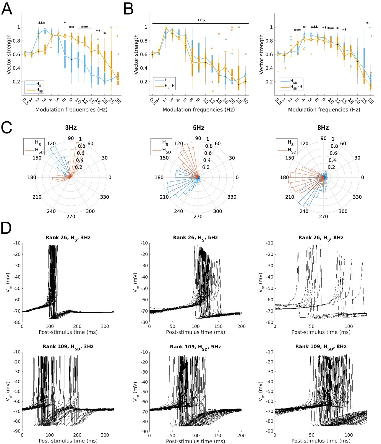
Firing precision and phase of models with modulated somatodendritic inputs.
(A) Firing precision (vector strength) across models with somatic H (blue) and somatodendritic H (orange) in control (without H block), across all modulation frequencies (F(1,15) = 9.378, p<0.001, n = 16; Huynd-Feldt correction). Boxplot annotations as per Figure 1G legend. (B) Vector strength across models with somatic H (HS, left) and somatodendritic H (HSD, right), in control (blue) and with H blocked (orange), across all modulation frequencies. Statistical test used was two-way repeated measures ANOVA for the populations of HS and HSD models between all modulation frequencies crossed with H block condition (HS: F(1,15) = 1.682, p=0.13, n = 16; HSD: F(1,15) = 4.45, p=0.009, n = 16; Huynd-Feldt correction reported for both tests). Boxplot annotations as per Figure 1G legend. (C) Firing phase histograms for models with somatic H (blue) and somatodendritic H (orange) for modulation frequencies of 3 Hz (left), 5 Hz (middle), and 8 Hz (right). (D) Overlay of Vm traces of all spikes for a sample somatic H model (top row) and somatodendritic H model (bottom row), cut and aligned with respect to the time of release from inhibition at 3 Hz (left), 5 Hz (middle), and 8 Hz (right).
Figure 4 with 1 supplement
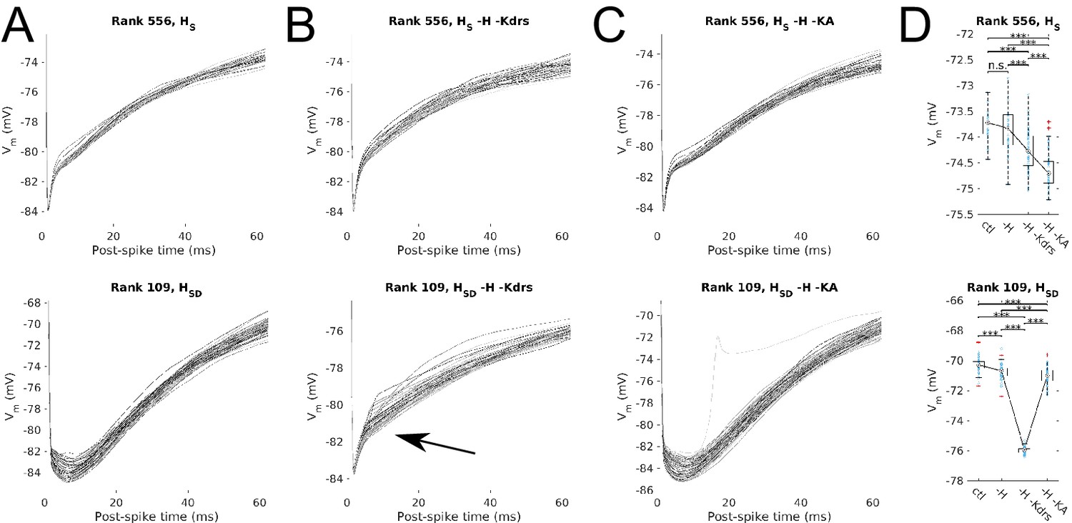
Post-spike Vm trajectories at 8 Hz modulation for models with Kdrs and KA blocked.
Overlays of the post-spike Vm trajectories plotted by aligning the post-spike Vm at spike peaks, for 8 Hz modulation simulations. Traces end halfway to the next 8 Hz theta cycle (62.5 ms) and are averaged for each model. One set of traces is shown per model, with each model’s averaged post-spike Vm trace given a different shade of grey to facilitate visualization. Cases shown are models with somatic H (HS, top) and somatodendritic H (HSD, bottom) in control (A), H and Kdrs blocked (B), and H and KA blocked (C). Arrow in (B) denotes where post-spike Vm trajectories in the HSD model changes to resemble that of an HS model with H and Kdrs block (see main text). (D) The distribution of averaged Vm values at the halfway point to the next theta cycle, i.e., the values shown at the end of each of the traces for the conditions shown, for the somatic H (top) and somatodendritic H (bottom) models. Statistical test used was 2-sample t-test with p<0.001 (***) and n.s. denoting not significant. n = 16 for each HS and HSD population.
Figure 4—figure supplement 1
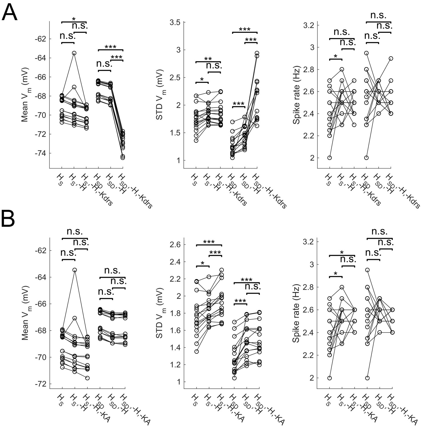
Effect of blocking H as well as Kdrs and/or KA on sub- and suprathreshold measures.
Models with control, H block (-H) and either Kdrs block (-H, -Kdrs) (A) or KA block (-H, -KA) (B) showing somatic Vm means (lef), fluctuations expressed as standard deviation (middle), and firing rates (right). Both models with somatic H (HS) and somatodendritic H (HSD) distributions are shown. Statistical test throughout was 2-sample t-test, with p<0.05 (*), p<0.001 (***), and n.s. denoting not significant. n = 16 for each population of models.
Figure 5
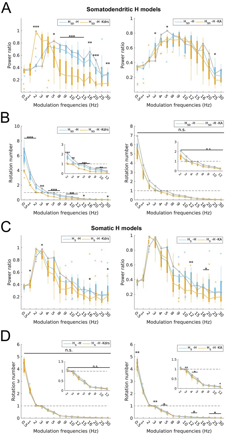
Changes to spiking recruitment in models with block of H and Kdrs or KA.
Power ratios (A) and rotation numbers (B) for somatodendritic H (HSD) models with either H and Kdrs blocked (left), or H and KA blocked (right). Power ratios (C) and rotation numbers (D) for somatic H (HS) models with either H and Kdrs blocked (left), or H and KA blocked (right). In all cases, the control condition is H blocked only, without additional Kdrs and KA block. The grey line depicts median values of corresponding cases without H block. Insets in rotation number plots in (B) and (D) show zoomed portion in the theta range (2–12 Hz). Statistical test used was repeated measures ANOVA for the relevant populations between all modulation frequencies crossed with H block condition ((A) -H -Kdrs: F(1,15) = 14.44, p<0.001, n = 12; -H -KA: F(1,15) = 4.20, p<0.001, n = 8; (B) -H -Kdrs: F(1,15) = 21.20, p=0.001, n = 12; -H -KA: F(1,15) = 2.4768, p=0.1576 (n.s.), n = 8; (C) -H -Kdrs: F(1,15) = 2.81, p=0.009, n = 16; -H -KA: F(1,15) = 2.43, p=0.03, n = 16; (D) -H -Kdrs: F(1,15) = 0.33, p=0.59, n = 16; -H -KA: F(1,15) = 6.51, p=0.02, n = 16; Huynd-Feldt correction reported for all tests). Boxplot annotations as per Figure 1G legend.
Figure 6 with 1 supplement
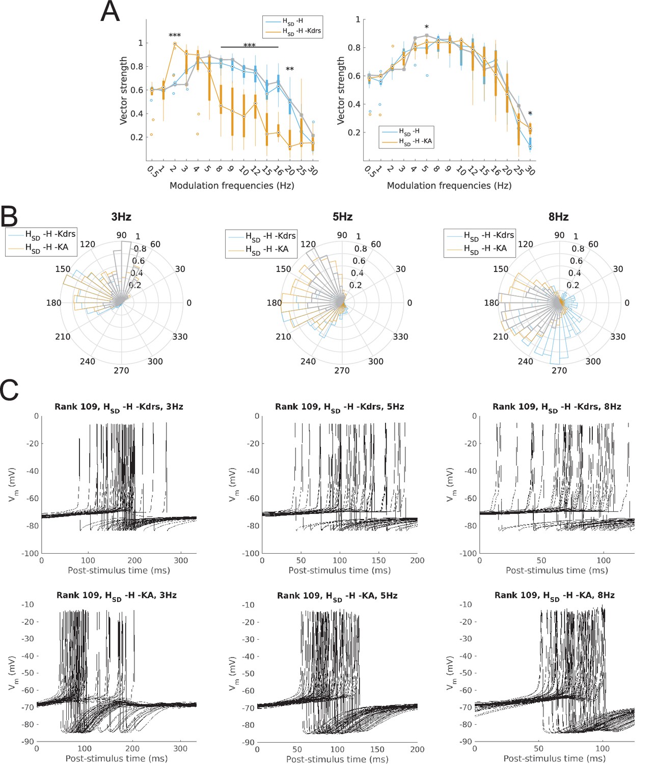
Changes to firing precision and phase in somatodendritic H models with block of H and Kdrs or KA.
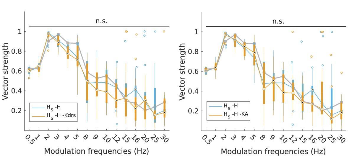
(A) Firing precision (vector strength) across somatodendritic H (HSD) models, with H and Kdrs blocked (blue) and with H and KA blocked (orange) across all modulation frequencies (F(1,15) = 16.00, p<0.001, n = 8; Huynd-Feldt correction). Boxplot annotations as per Figure 1G. (B) Vector strength across HSD models with only H blocked (blue, -H) and with H and Kdrs blocked (left, orange, -H -Kdrs) and H and KA blocked (right, orange, -H -KA), across all modulation frequencies. The grey line depicts median values of corresponding cases without H block (control). Statistical test used was two-way repeated measures ANOVA test for the population of -H -Kdrs and -H -KA models between all modulation frequencies crossed with H and Kdrs/KA blocked condition (-H -Kdrs: F(1,15) = 18.739, p<0.001, n = 12; -H -KA: F(1,15) = 2.83, p=0.01, n = 8; Huynd-Feldt correction reported for both tests). Boxplot annotations as per Figure 1G. (C) Firing phase histograms for HSD models with H and Kdrs blocked (blue) and H and KA blocked (orange) for modulation frequencies of 3 Hz (left), 5 Hz (middle), and 8 Hz (right). In all cases, the control condition is H blocked only, without additional Kdrs and KA block. (D) Overlay of Vm traces of all spikes for an example HSD model with H and Kdrs blocked (top row) and H and KA blocked (bottom row), cut and aligned with respect to the time of release from inhibition at 3 Hz (left), 5 Hz (middle), and 8 Hz (right).
Figure 6—figure supplement 1
Changes to firing precision in somatic H models with block of H and Kdrs or KA.
Vector strength across somatic H models with only H blocked (blue, -H) and with H and Kdrs blocked (left, orange, -H -Kdrs) and H and KA blocked (right, orange, -H -KA), across all modulation frequencies (n.s. denotes not significant, n = 16 in both -H -Kdrs and -H -KA populations). The grey line depicts median values of corresponding cases without H block (control).
Figure 7
Effects on spiking resonance of simulating cAMP modulation of H channels.
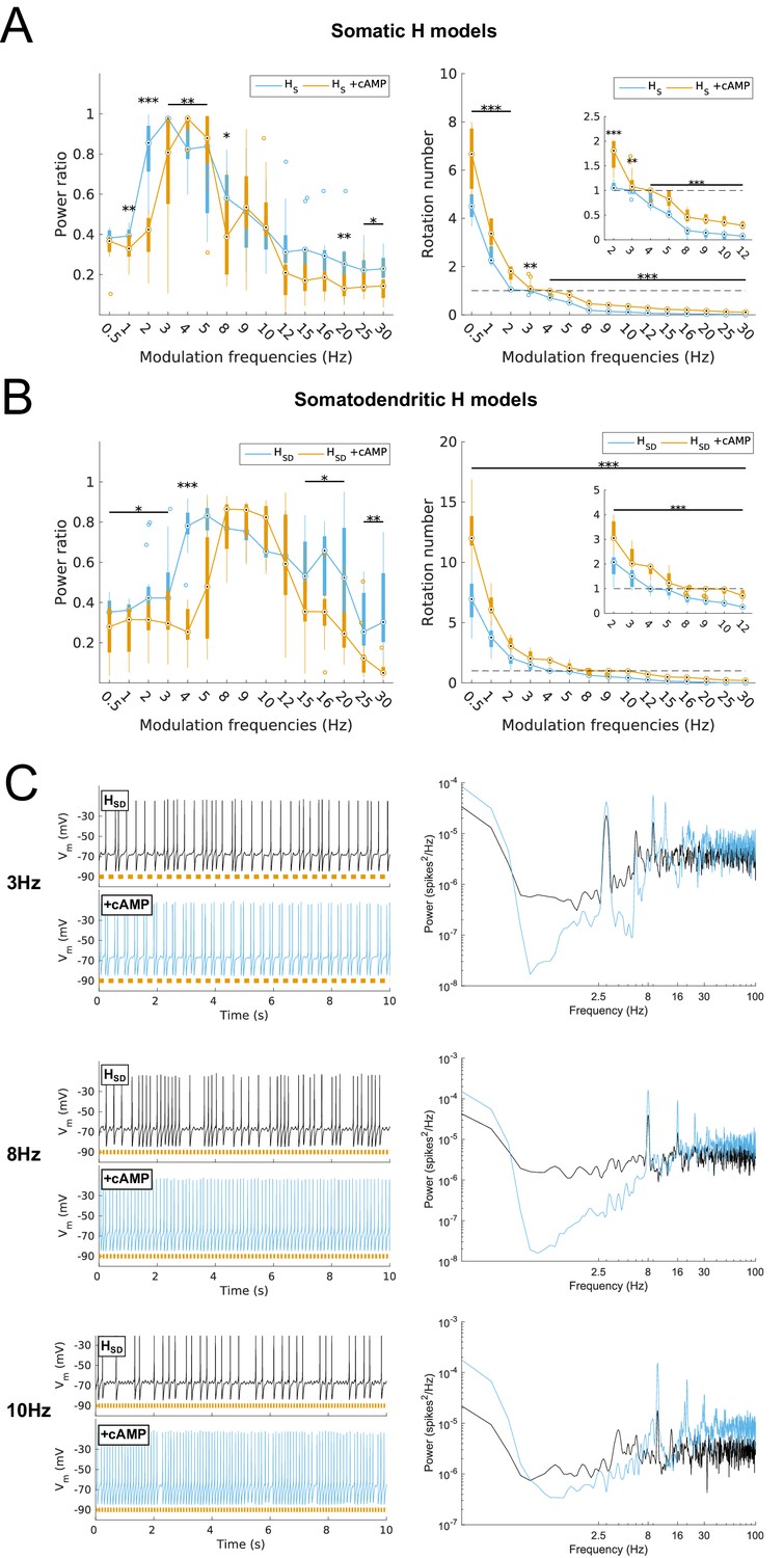
(A, B) Power ratios (left) and rotation numbers (right) under different modulation frequencies for somatic H models (B, HS) and somatodendritic H models (C, HSD) in control and cAMP (‘+cAMP’) conditions. Insets in rotation number plots show zoomed portion in the theta range (2–12 Hz). Statistical test used was repeated measures ANOVA for the populations of HS and HSD models between all modulation frequencies crossed with cAMP condition (power ratios HS: F(1,15) = 18.66, p<0.001, n = 16; HSD: F(1,15) = 5.16, p=0.003, n = 16; rotation numbers HS: F(1,15) = 79.23, p<0.001, n = 16; HSD: F(1,15) = 59.52, p<0.001, n = 16; Huynd-Feldt correction reported for all tests). Boxplot annotations as per Figure 1G legend. (C) Somatic Vm traces for an example model in control (black) and cAMP (blue) under various modulation conditions (top – no modulation; middle – 3 Hz modulation; bottom – 8 Hz modulation). With modulated inputs, orange bars at bottom denote phase of peak modulation at the specified frequency (see Materials and methods). Power spectrum density (PSD) plots shown to the right of each set of output traces.
Figure 8
Firing precision and phase of models with cAMP modulation of H channels.
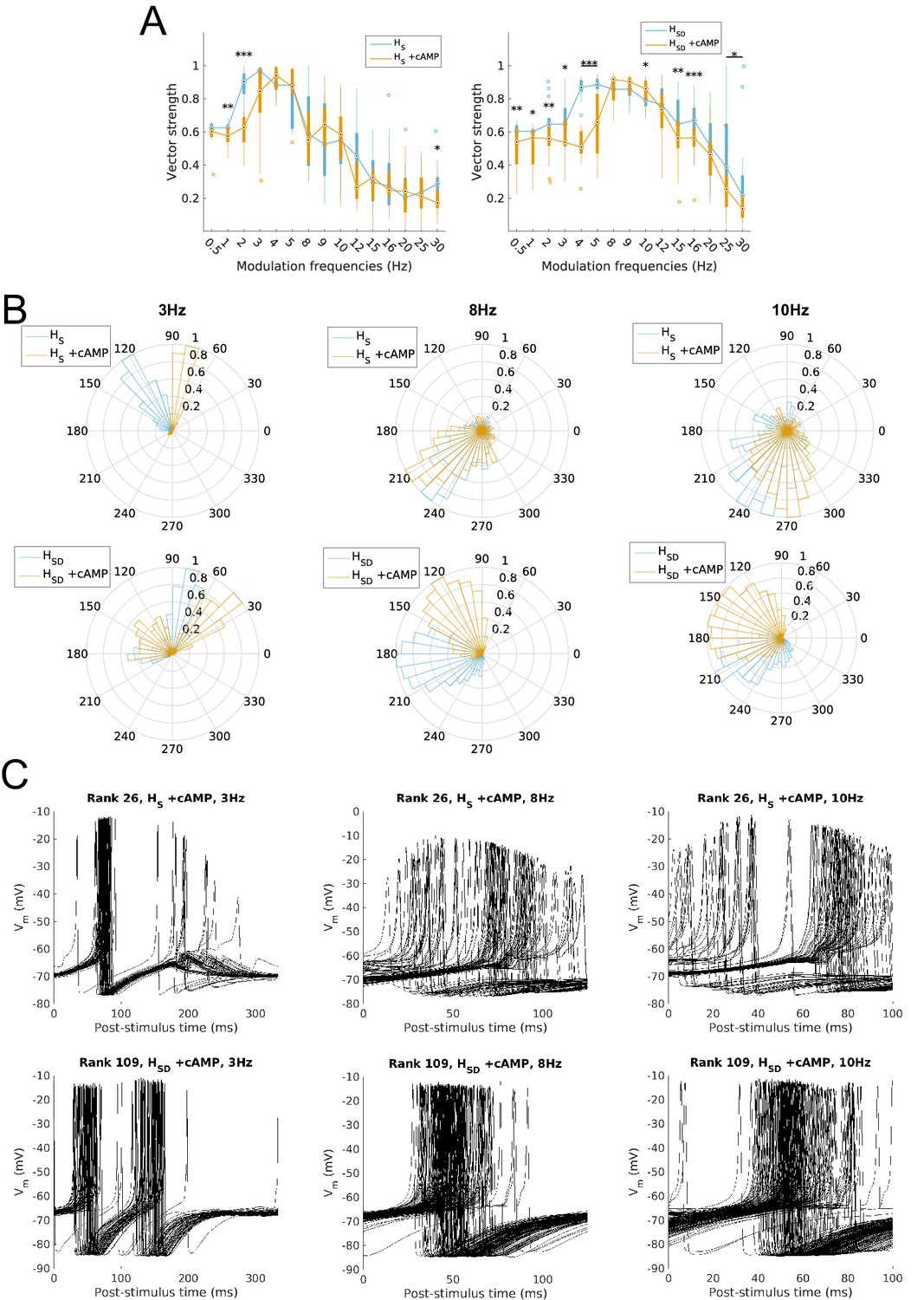
(A) Vector strength across models with somatic H (HS, left) and somatodendritic H (HSD, right), in control (blue) and with cAMP (orange) conditions, across all modulation frequencies. Statistical test used was two-way repeated measures ANOVA test for the populations of HS and HSD models between all modulation frequencies crossed with H blocked condition (HS: F(1,15) = 4.20, p=0.003, n = 16; HSD: F(1,15) = 6.38, p<0.001, n = 16; Huynd-Feldt correction reported for both tests). Boxplot annotations as per Figure 1G legend. (B) Firing phase histograms for models under cAMP condition with somatic H (top) and somatodendritic H (bottom), for control (blue) and cAMP (orange) conditions, and modulation frequencies of 3 Hz (left), 8 Hz (middle), and 10 Hz (right). (C) Overlay of Vm traces of all spikes for an example somatic H model with cAMP (top row) and somatodendritic H model with cAMP (bottom row), cut and aligned with respect to time of release from inhibition at 3 Hz (left), 8 Hz (middle), and 10 Hz (right).
Author response image 1
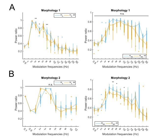
Partitioning of spiking responses of O-LM models into high and low theta when separately analyzing models with different morphologies.
Models with morphology 1 (A) or morphology 2 (B) and HS (left) vs HSD (right) distributions. Statistical test used was repeated measures ANOVA for the populations of HS and HSD models between all modulation frequencies crossed with H condition (morphology 1 HS: F(1,15) = 2.23, p=0.01, n=8; morphology 1 HSD: F(1,15) = 0.75, p=0.64, n=5; morphology 2 HS: F(1,15) = 2.31, p=0.37, n=8; morphology 2 HSD: F(1,15) = 2.60, p=0.02, n=7; Huynd-Feldt correction reported for all tests). Boxplot annotations as per Figure 1G legend. Note that not enough models with morphology 2 and somatic H completed the modulation simulations under 48 hours for frequencies above 12 Hz (B, left) to be able to perform a repeated measures ANOVA test; thus, only simulations with modulation frequencies 12 Hz and below are included in the analysis.
Tables
Table 1
Parameter values for models used in this work. Parameters taken from the database include the ion channel maximum conductance densities and the morphology (cell 1 or cell 2; see Figure 1B), H channel distribution (HS – somatic H; HSD – somatodendritic H, uniformly distributed). Units for maximum conductance densities are in pS/µm2.
| Somatic H models | ||||||||||||||||
|---|---|---|---|---|---|---|---|---|---|---|---|---|---|---|---|---|
| Rank | 326 | 556 | 613 | 620 | 689 | 723 | 755 | 769 | 26 | 31 | 39 | 43 | 45 | 60 | 67 | 68 |
| cell | 1 | 1 | 1 | 1 | 1 | 1 | 1 | 1 | 2 | 2 | 2 | 2 | 2 | 2 | 2 | 2 |
| hD | 0 | 0 | 0 | 0 | 0 | 0 | 0 | 0 | 0 | 0 | 0 | 0 | 0 | 0 | 0 | 0 |
| H | 0.5 | 0.5 | 0.5 | 0.5 | 0.5 | 0.5 | 0.5 | 0.5 | 0.5 | 0.5 | 0.5 | 0.5 | 0.5 | 0.5 | 0.5 | 0.5 |
| Nad | 117 | 117 | 117 | 117 | 117 | 117 | 117 | 117 | 117 | 117 | 117 | 117 | 117 | 117 | 117 | 117 |
| Nas | 107 | 220 | 107 | 220 | 107 | 60 | 60 | 107 | 107 | 107 | 107 | 60 | 107 | 60 | 107 | 107 |
| Kdrf | 215 | 215 | 215 | 215 | 215 | 215 | 215 | 215 | 215 | 215 | 215 | 215 | 215 | 215 | 215 | 215 |
| Kdrs | 2.3 | 2.3 | 2.3 | 2.3 | 2.3 | 2.3 | 2.3 | 2.3 | 2.3 | 2.3 | 2.3 | 2.3 | 2.3 | 2.3 | 2.3 | 2.3 |
| KA | 2.5 | 32 | 32 | 32 | 2.5 | 32 | 2.5 | 2.5 | 2.5 | 32 | 2.5 | 2.5 | 32 | 32 | 32 | 2.5 |
| CaT | 2.5 | 5 | 2.5 | 5 | 2.5 | 5 | 5 | 1.25 | 1.25 | 5 | 2.5 | 2.5 | 5 | 2.5 | 2.5 | 5 |
| CaL | 50 | 50 | 25 | 25 | 25 | 25 | 25 | 25 | 25 | 25 | 25 | 25 | 50 | 12.5 | 50 | 50 |
| AHP | 11 | 5.5 | 2.75 | 5.5 | 5.5 | 5.5 | 11 | 5.5 | 11 | 5.5 | 11 | 2.75 | 2.75 | 2.75 | 2.75 | 11 |
| M | 0.375 | 0.375 | 0.375 | 0.375 | 0.75 | 0.375 | 0.375 | 0.75 | 0.375 | 0.375 | 0.375 | 0.375 | 0.375 | 0.375 | 0.375 | 0.375 |
| Somatodendritic H models | ||||||||||||||||
|---|---|---|---|---|---|---|---|---|---|---|---|---|---|---|---|---|
| Rank | 225 | 356 | 913 | 1230 | 1520 | 2050 | 2173 | 2286 | 6 | 34 | 37 | 49 | 57 | 92 | 96 | 109 |
| cell | 1 | 1 | 1 | 1 | 1 | 1 | 1 | 1 | 2 | 2 | 2 | 2 | 2 | 2 | 2 | 2 |
| hD | 1 | 1 | 1 | 1 | 1 | 1 | 1 | 1 | 1 | 1 | 1 | 1 | 1 | 1 | 1 | 1 |
| H | 0.1 | 0.1 | 0.1 | 0.1 | 0.1 | 0.1 | 0.1 | 0.1 | 0.1 | 0.1 | 0.1 | 0.1 | 0.1 | 0.1 | 0.1 | 0.1 |
| Nad | 230 | 230 | 230 | 230 | 230 | 230 | 230 | 230 | 230 | 230 | 230 | 230 | 230 | 230 | 230 | 230 |
| Nas | 107 | 220 | 107 | 60 | 60 | 60 | 107 | 220 | 60 | 107 | 107 | 107 | 107 | 60 | 60 | 107 |
| Kdrf | 506 | 506 | 506 | 506 | 506 | 506 | 506 | 506 | 506 | 506 | 506 | 506 | 506 | 506 | 506 | 506 |
| Kdrs | 42 | 42 | 42 | 42 | 42 | 42 | 42 | 42 | 42 | 42 | 42 | 42 | 42 | 42 | 42 | 42 |
| KA | 2.5 | 2.5 | 2.5 | 2.5 | 2.5 | 2.5 | 2.5 | 2.5 | 2.5 | 2.5 | 2.5 | 2.5 | 2.5 | 2.5 | 32 | 32 |
| CaT | 1.25 | 2.5 | 1.25 | 1.25 | 2.5 | 1.25 | 2.5 | 1.25 | 5 | 5 | 1.25 | 5 | 1.25 | 2.5 | 1.25 | 2.5 |
| CaL | 25 | 50 | 50 | 25 | 12.5 | 25 | 25 | 25 | 25 | 25 | 12.5 | 12.5 | 25 | 50 | 25 | 50 |
| AHP | 5.5 | 2.75 | 5.5 | 2.75 | 5.5 | 5.5 | 5.5 | 5.5 | 2.75 | 2.75 | 2.75 | 2.75 | 11 | 5.5 | 5.5 | 5.5 |
| M | 0.75 | 0.375 | 0.75 | 0.375 | 0.375 | 0.375 | 0.375 | 0.75 | 0.375 | 0.375 | 0.75 | 0.375 | 0.375 | 0.375 | 0.375 | 0.375 |
Table 2
Additional parameters re-fitted as per Sekulić et al. (2015) to improve h-channel activation kinetics and passive properties. Shown here are the specific membrane resistivity, Rm, the specific membrane capacitance, Cm., and bias current needed to keep model somatic Vm at −74 mV as per the experimental data used for fitting. However, the bias current was not used in any of the high-conductance synaptic input simulations. For the fitted H channel steady-state activation function, see Figure 1—figure supplement 1.
| Somatic H models | Somatodendritic H models | ||||||||
|---|---|---|---|---|---|---|---|---|---|
| Rank | Cell | Rm (Ω·cm2) | Cm (µF/cm2) | Ibias (pA) | Rank | Cell | Rm (Ω·cm2) | Cm (µF/cm2) | Ibias (pA) |
| 326 | 1 | 80,932 | 0.5119 | −6.79 | 225 | 1 | 138,328 | 0.6603 | −10.3 |
| 556 | 1 | 90,251 | 0.4981 | −0.932 | 356 | 1 | 122,359 | 0.6515 | −11.3 |
| 613 | 1 | 89,118 | 0.5282 | −1.57 | 913 | 1 | 130,845 | 0.6524 | −10.3 |
| 620 | 1 | 90,099 | 0.5025 | −0.932 | 1230 | 1 | 131,079 | 0.6574 | −11.2 |
| 689 | 1 | 79,102 | 0.5069 | −8.19 | 1520 | 1 | 130,763 | 0.6520 | −10.5 |
| 723 | 1 | 90,289 | 0.4950 | −0.846 | 2050 | 1 | 131,588 | 0.6528 | −10.5 |
| 755 | 1 | 80,939 | 0.5058 | −6.83 | 2173 | 1 | 129,748 | 0.6505 | −10.5 |
| 769 | 1 | 79,183 | 0.5057 | −8.16 | 2286 | 1 | 130,703 | 0.6547 | −10.4 |
| 26 | 2 | 64,872 | 1.046 | −15.2 | 6 | 2 | 71,586 | 1.086 | −7.0 |
| 31 | 2 | 68,312 | 1.058 | −12.3 | 34 | 2 | 68,585 | 1.083 | −7.04 |
| 39 | 2 | 63,968 | 1.060 | −15.2 | 37 | 2 | 71,079 | 1.086 | −6.9 |
| 43 | 2 | 63,041 | 1.042 | −16.4 | 49 | 2 | 71,129 | 1.083 | −7.04 |
| 45 | 2 | 66,584 | 1.058 | −12.7 | 57 | 2 | 71,750 | 1.082 | −5.76 |
| 60 | 2 | 67,959 | 1.048 | −12.6 | 92 | 2 | 71,891 | 1.081 | −6.56 |
| 67 | 2 | 68,083 | 1.047 | −12.7 | 96 | 2 | 72,746 | 1.066 | −2.13 |
| 68 | 2 | 64,339 | 1.053 | −15.2 | 109 | 2 | 75,364 | 1.061 | −2.18 |
Download links
A two-part list of links to download the article, or parts of the article, in various formats.
Downloads (link to download the article as PDF)
Open citations (links to open the citations from this article in various online reference manager services)
Cite this article (links to download the citations from this article in formats compatible with various reference manager tools)
Computational models of O-LM cells are recruited by low or high theta frequency inputs depending on h-channel distributions
eLife 6:e22962.
https://doi.org/10.7554/eLife.22962


