Wiring variations that enable and constrain neural computation in a sensory microcircuit
- Harvard Medical School, United States
Figures
Figure 1 with 6 supplements
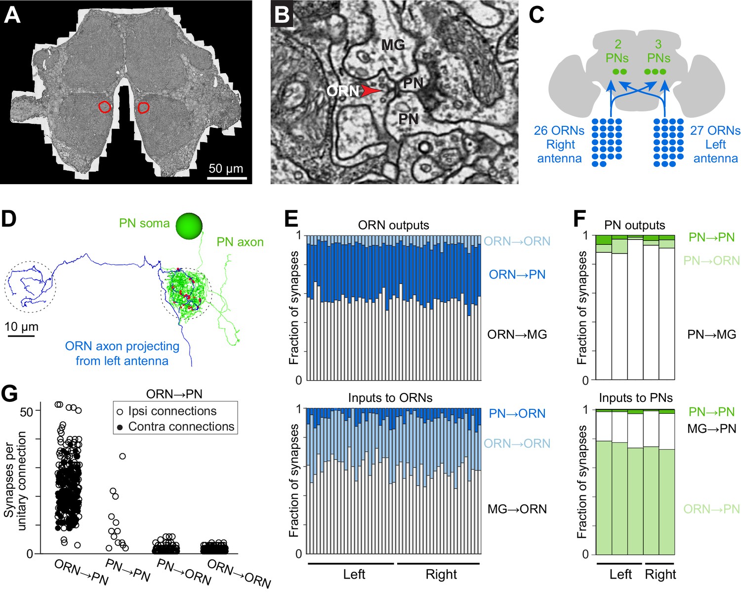
Cells and connections comprising the glomerular micro-circuit.
(A) Electron micrograph of a frontal section (76,000 × 58,000 pixels) from the anterior portion of the brain. Glomerulus DM6 is outlined. (B) Zoomed-in view of a synapse. Red arrowhead demarcates a presynaptic specialization (T-bar). The long edge of the image measures 2 µm. (C) Schematic of reconstructed cells. All ORNs and PNs within glomerulus DM6 were fully reconstructed. Not shown in this schematic are multi-glomerular neurons (cells that interconnect different glomeruli), which were not fully reconstructed. (D) 3-D rendering of a single ORN→PN cell pair viewed frontally. The ORN axon (blue) makes multiple synapses (red) onto the PN dendrite (green). The approximate region occupied by the DM6 glomerulus is circled with dashed lines. The PN cell body is represented as a sphere for display purposes. (E) Top: synapses made by ORNs, expressed as a fraction of each ORN’s total pool of output synapses. Bottom: synapses received by ORNs, expressed as a fraction of each ORN’s total pool of input synapses. ‘MG’ denotes multiglomerular neurons. (F) Synapses made by PNs and received by PNs, normalized in the same way. (G) Number of synapses between connected pairs of cells, sorted by connection type. Each symbol represents a unitary connection.
Figure 1—figure supplement 1
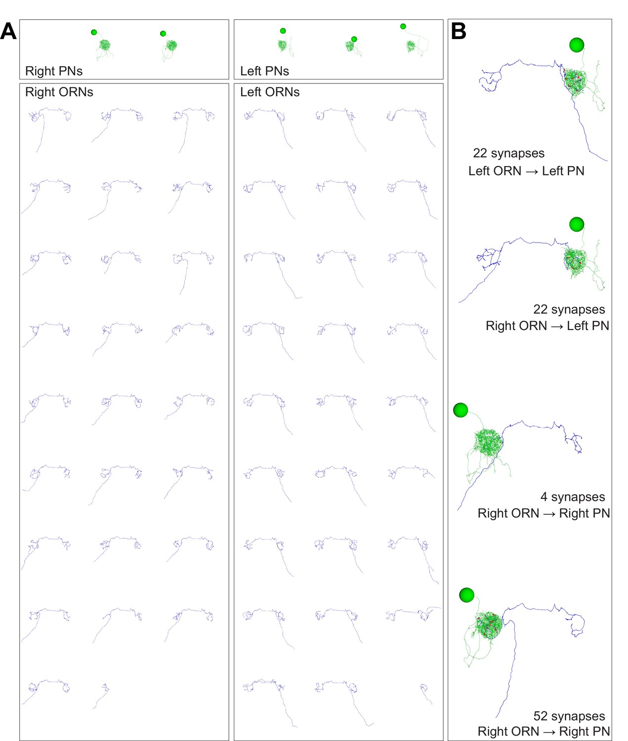
Anatomical gallery: ORNs, PNs, and connected pairs.
Renderings of neuron reconstructions in glomerulus DM6 from the frontal perspective. Cell bodies, axons, dendrites and synapses colored as in Figure 1D. Large balls represent cell bodies (9 μm in diameter) and small red balls represent ORN output synapses. The axonal projection of PNs are omitted. (A) All PNs and ORNs. (B) Examples of connected ORN-PN pairs.
Figure 1—figure supplement 2
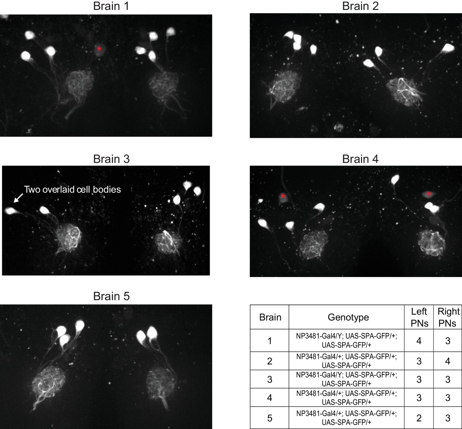
Variations in the number of PNs in glomerulus DM6.
By counting Gal4-expressing PNs in a glomerulus, we can obtain a lower bound on the number of PNs that reside in that glomerulus. No Gal4 line has been identified which drives expression exclusively in DM6 PNs. However, the NP3481-Gal4 line drives expression in DM6 PNs along with PNs in several other glomeruli (total count is 9.5 PNs on average [Tanaka et al., 2012]). In order to limit a fluorescent marker to DM6 PNs alone, we used NP3481-Gal4 to drive expression of photoactivatible GFP (UAS-SPA) (Datta et al., 2008), and we used 2-photon excitation to specifically photoactivate GFP within the DM6 glomerulus. Because the dendritic arbor of each PN typically ramifies throughout the entire glomerulus, photoactivating within a large fraction of the glomerulus should label each Gal4+ PN. In five experiments, we photoactivated both the right and left copies of DM6. Images shown here are maximum-intensity projections of confocal stacks imaged in a coronal plane (dorsal is up; red asterisks denote dim somata that were not photoactivated and that are not associated with DM6, based on inspection of the 3D stack). Most frequently we found three PNs per glomerulus, but we also occasionally found four or two PNs. The number of PNs was often different on the two sides of the same brain, but there was no systematic difference between right and left. This result implies that the number of Gal4+ DM6 PNs can vary, consistent with variable counts in other glomeruli in the number of Gal4+ PNs (Tanaka et al., 2004; Grabe et al., 2016). Our EM reconstruction implies that at least some of this variability is due to true variation in PN counts, and is not merely due to variations in Gal4 expression patterns.
Figure 1—figure supplement 3

Images of representative synapses connecting different cell types.
Example electron micrographs of: (A–D) ORN→PN synapses, (E–H) PN→PN synapses, (I–L) PN→ORN synapses, (M–P) ORN→ORN synapses. Note that each synapse spanned multiple sections. Red arrowheads point toward presynaptic specializations. Scale bar in (P) is 500 nm.
Figure 1—figure supplement 4

Connectivity matrix of ORNs and PNs in glomerulus DM6.
Adjacency matrix color coded by the number of synapses connecting pre- and postsynaptic pairs. Neurons are sorted within cell type (ORN or PN) by their left/right identity. A neuron’s position in the matrix is the same as in Figure 1—figure supplement 4—source data 1.
-
Figure 1—figure supplement 4—source data 1
Matrix of ORN-PN connectivity.
This comma-separated values file contains the number of synapses connecting every pair of reconstructed DM6 ORNs and PNs. Neurons are sorted within cell type (ORN or PN) by their left/right identity. A neuron’s position in the matrix is the same as in Figure 1—figure supplement 4.
- https://doi.org/10.7554/eLife.24838.007
Figure 1—figure supplement 5
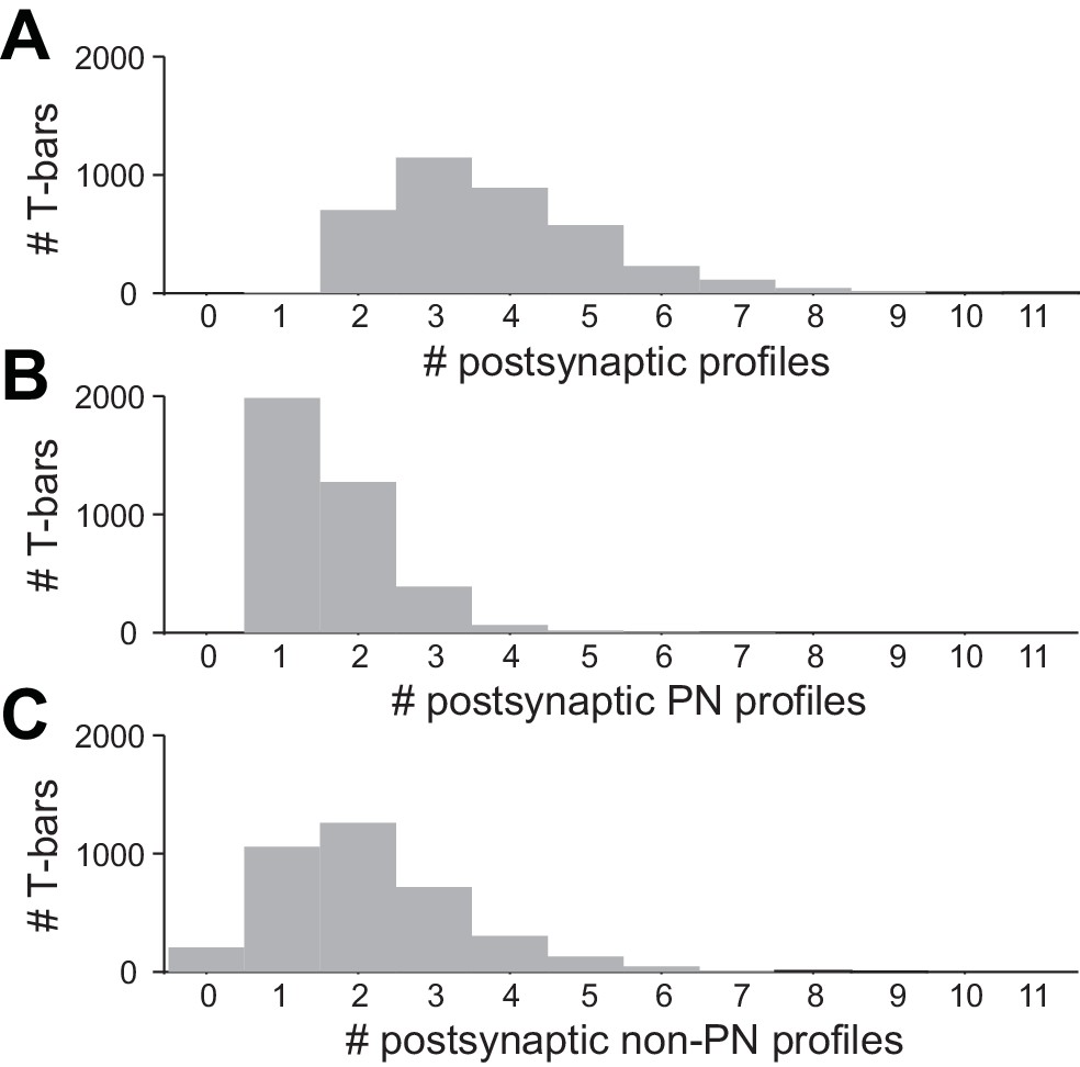
Multiplicity of postsynaptic profiles.
(A) Histogram of the number of postsynaptic profiles per ORN T-bar. Only ORN T-bars that contacted at least one PN were considered here. (B) Data on the same T-bars, for postsynaptic PN profiles only. (C) Data on the same T-bars, for postsynaptic non-PN profiles only.
Figure 1—figure supplement 6
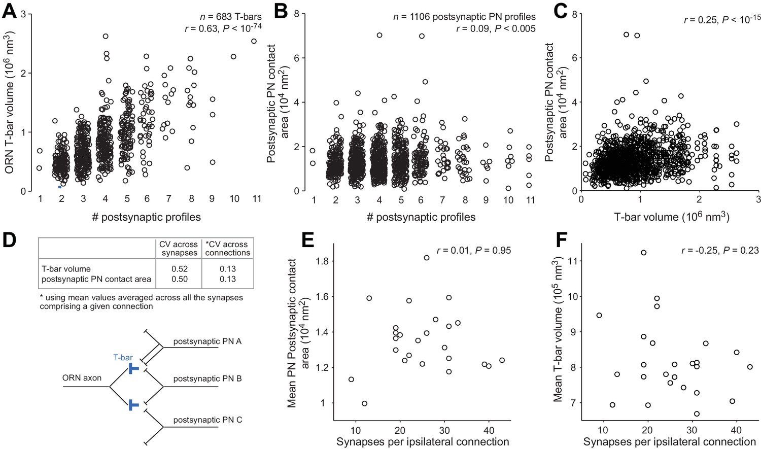
T-bar volume and postsynaptic contact area.
We randomly selected 5 ORNs in the left antenna and 5 ORNs in the right antenna. Each of these ORNs contacted all 5 DM6 PNs. We measured the volume of each T-bar formed by these 10 ORNs, including only the T-bars that contacted at least one PN (n = 683 ORN T-bars). We also measured the area of all postsynaptic PN profiles contacting these 683 T-bars (n = 1106 PN profiles; note that some T-bars contact more than one PN, and occasionally a T-bar will contact the same PN at two sites). (A) ORN T-bar volume is significantly correlated with the number of postsynaptic profiles at that T-bar. (B) Postsynaptic PN contact area is significantly correlated with the number of postsynaptic profiles at that T-bar, although the correlation is weak. (C) Postsynaptic PN contact area is significantly correlated with T-bar volume. Note that some T-bars are counted more than once because they contact multiple PN profiles. (D) The coefficient of variation (CV) of T-bar volume and postsynaptic PN contact area. Averaging across the synapses contributing to a given connection substantially decreases CVs. (E) Mean postsynaptic PN contact area (averaged across synapses in the same connection) is not correlated with the number of synapses per connection. (F) Mean T-bar volume (averaged across synapses in the same connection) is not correlated with the number of synapses per connection.
Figure 2
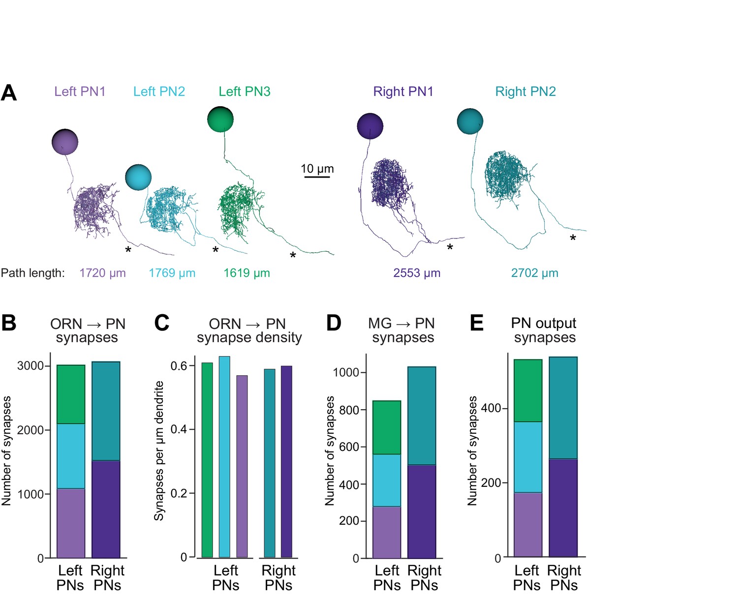
Connectivity compensates for a missing cell.
(A) Skeletonized 3-D renderings of reconstructed PNs. Cells are viewed parasagittally from the left. For each cell, the total path length of all dendrite segments is indicated; note that PNs on the right side of the brain have longer path lengths. Axons are indicated with asterisks. (B) Synapses received by each PN from ORNs. (C) Number of ORN→PN synapses for each PN, normalized for the total path length of each PN’s dendrites. (D) Synapses received by each PN from multi-glomerular (MG) neurons. (E) Output synapses made by each PN within the DM6 glomerulus.
Figure 3
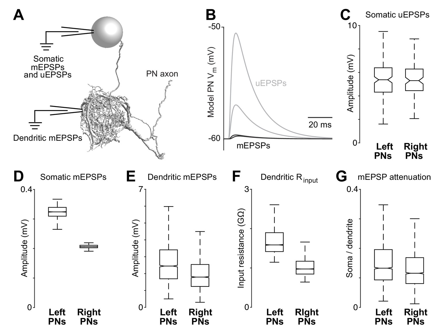
Dendritic arbor size equalizes average unitary responses.
(A) Volumetric 3-D rendering of an EM reconstructed PN dendrite. (The cell body is represented as a sphere for display purposes.) Compartmental models fit to ultrastructural and electrophysiological data were used to simulate the voltage responses of each PN to synaptic input from ORNs. Synaptic conductances were simulated in the PN dendrite, and voltage responses were recorded in either the cell body or in the dendritic compartment where a given synapse was located. Each of the five reconstructed PNs was modeled in this way. (B) Example voltage responses recorded at the cell body of a model PN. A miniature EPSP (mEPSP) is the response to a quantum of neurotransmitter. A unitary EPSP (uEPSP) is the response to one spike in a single presynaptic axon, i.e. the combined effect of all the mEPSPs generated by that axon. Shown here are the largest and smallest mEPSPs and uEPSPs in this PN. In the model, a spike always produces the same conductance at all synapses, and so variations in mEPSP amplitude must be due to variations in the position of synapses on the dendrite. (C) There is no left-right difference in the amplitude of uEPSPs, measured at the cell body of each PN (computed across unitary ORN→PN connections, p>0.7, permutation test, n = 156 left and 104 right unitary connections). Here and elsewhere, box plots show median, 25th percentile and 75th percentile. Whiskers indicate 2.7 SDs (99.3% coverage of normally distributed data); for clarity, outliers beyond the whiskers are not displayed; notches indicate 95% confidence intervals. (D) There is a significant left-right difference in the amplitude of mEPSPs, measured at the cell body of the PN (computed across all ORN→PN synapses, p<0.0001, permutation test, n = 3013 left and 3066 right synapses). (E) There is a significant left-right difference in the amplitude of mEPSPs, measured at the site of each synapse in the dendrite (computed across all ORN→PN synapses, p<0.0001, permutation test). (F) There is a significant left-right difference in dendritic input resistance, measured across all model cables (computed across all PN cables, p<0.0001, permutation test, n = 5520 left and 6048 right cables). (G) There is a significant left-right difference in the attenuation of mEPSPs as they travel from the site of the synapse to the soma (ratio of somatic to dendritic amplitude computed across all ORN→PN synapses, p<0.0001, permutation test).
Figure 4 with 1 supplement
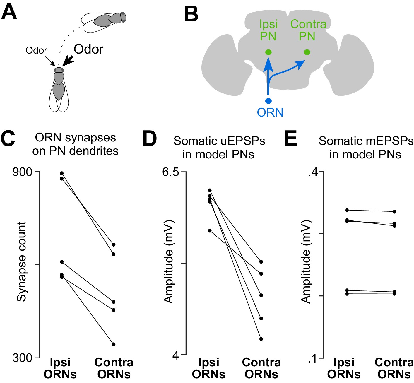
A basis for odor lateralization behavior in ORN wiring.
(A) Flies turn toward lateralized odor stimuli, a behavioral response termed osmotropotaxis. (B) Schematic of an ORN axon projecting bilaterally. Note that ipsi and contra are defined relative to the location of the ORN cell body. Unitary EPSPs in PNs driven by ipsilateral ORNs are systematically larger than those driven by contralateral ORNs (Gaudry et al., 2013). Successful odor lateralization requires that ipsi- and contralateral connections are systematically different. (C) PNs receive significantly more synapses from ipsilateral ORNs than from contralateral ORNs. Each connected pair of points represents a PN (p=0.0032, paired-sample t-test, n = 5 PNs). These 5 PNs collectively have 133 ipsi and 132 contra connections. (D) There is a significant ipsi-contra difference in mean modeled uEPSP amplitudes. Each connected pair of points represents a PN, with values averaged across all the connections received by that PN (p=0.0059, paired-sample t-test, n = 5 PNs). (E) There is no ipsi-contra difference in modeled mEPSP amplitudes. Each connected pair of points represents a PN, with values averaged over all the synapses received by that PN (p>0.05, paired-sample t-test, n = 5 PNs). These 5 PNs collectively have 3504 ipsi and 2575 contra synapses).
Figure 4—figure supplement 1
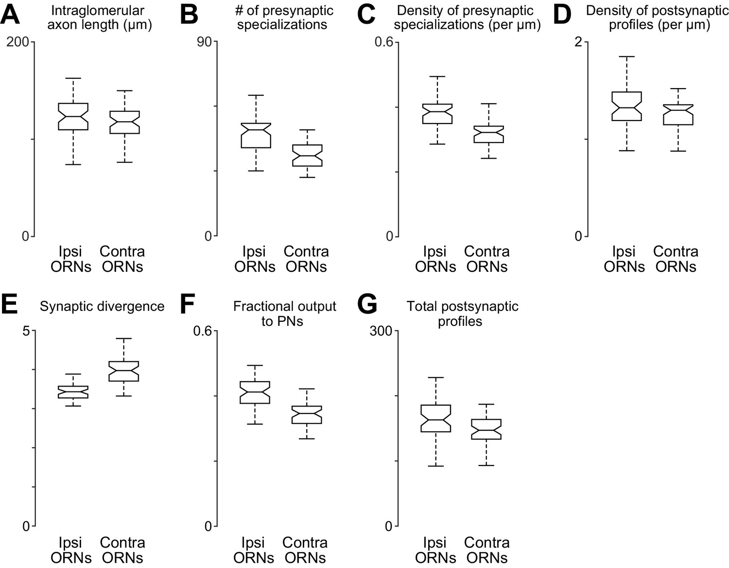
Comparing anatomical features of ipsi- and contralateral ORN axons.
(A) Total path length of each ORN axon within DM6 (p>0.11, permutation test, n = 106, because the 52 bilateral axons were each counted two times, and the two unilateral 2 axons were each counted one time). For each axon, we identified the first node upstream (proximal) to all synapses within the glomerulus, and then we computed the sum of the Euclidean distance between all connected nodes downstream from that node. (B) Total number of presynaptic specializations (T-bars) for each ORN axon within DM6 (p<0.0001, permutation test). (C) Density of presynaptic specializations (T-bars) for each ORN axon within DM6 (p<0.0001, permuta tion test). For each axon, the total number of T-bars was divided by the total cable length. (D) Postsynaptic profile density (p<0.025, permutation test). We counted the number of cellular profiles postsynaptic to each axon (the number of outgoing edges) within DM6, and then divided this by the total path length of the axon in that glomerulus. (E) Synaptic divergence (polyady) (p<0.0001, permutation test). We counted the number of profiles postsynaptic to each axon in DM6 and divided this by the number of presynaptic specializations (T-bars) in that axon in that glomerulus. (F) Fraction of output to PNs (P 0.0001, permutation test). This is the fraction of the profiles postsynaptic to each axon in DM6 that are PN profiles. (G) Total number of postsynaptic profiles (p<0.002, permutation test). This is the number of profiles postsynaptic to each axon.
Figure 5 with 1 supplement
Wiring inequalities among sister ORNs.
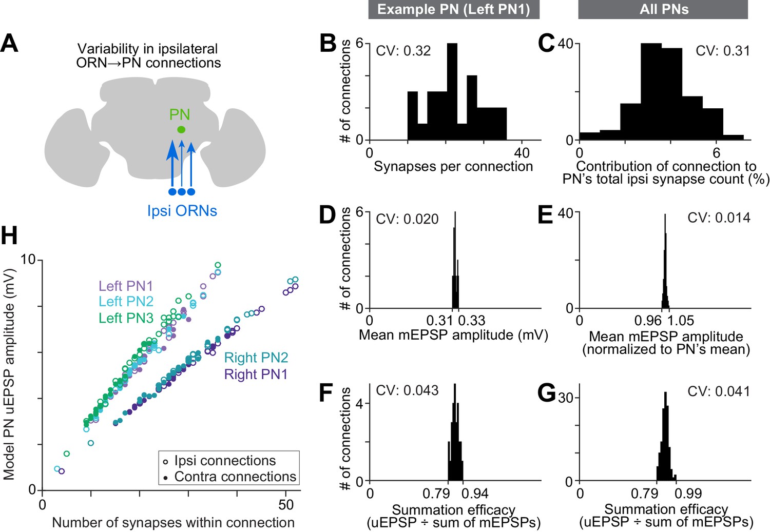
(A) Schematic of ORNs connected to a PN with different numbers of synapses. Arrow size represents the number of synapses each ORN forms on an ipsilateral PN dendrite. (B–G) Histograms showing variation among ipsilateral ORN→PN connections. The histograms are horizontally scaled so that the means of all distributions are aligned, in order to an enable a visual comparison of CVs. (B) Number of synapses that each ipsilateral ORN makes onto left PN1. (C) Analogous to (B) but pooled across all PNs. To enable pooling, we first normalize the number of synapses made by each ipsilateral ORN to the total number of ipsilateral ORN input synapses a PN receives. This yields the percentage contribution of each ORN to the ipsilateral synapse pool. The mean of this value is relatively consistent across the five PNs (0.037, 0.037, 0.037, 0.039, and 0.039), but there is a large variation within each PN. (D) Mean mEPSP amplitude for connections made by ipsilateral ORNs onto left PN1. At each unitary connection, the mean mEPSP amplitude is computed across all the synapses that contribute to that connection. This value is relatively consistent across unitary connections. (E) Analogous to (D) but pooled across all PNs. Each mEPSP value is normalized to the grand average for that PN. This value is consistent across all unitary connections, both within and across PNs. (F) Summation efficacy at connections made by ipsilateral ORNs onto left PN1. Summation efficacy is computed as the amplitude of the connection’s uEPSP, divided by the linearly summed amplitudes of all the mEPSPs that comprise the connection. Again, this value is relatively consistent across unitary connections. (G) Same as (F) but pooled across all PNs. (H) Correlation between synapse number per connection and uEPSP amplitude. Each data point is a unitary connection (n = 260), with ipsilateral (unfilled) and contralateral (filled) connections indicated. For each PN, there is a strong and significant correlation (Pearson’s r ranges from 0.993 to 0.999; P ranges from 9.78 × 10−48 to 1.34 × 10−65 after Bonferroni-Holm correction for multiple comparisons, m = 5 tests).
Figure 5—figure supplement 1
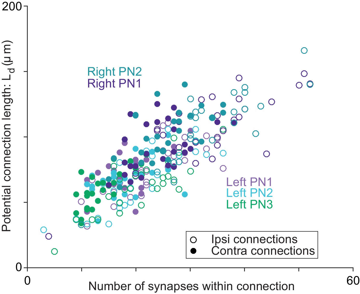
Axon-dendrite proximity correlates with the number of synapses per ORN→PN connection.
For each ORN-PN connection (n = 260), we measured the ‘potential connection length’ (Ld) as the total path length of the PN dendrite within 500 nm of the ORN axon (Lee et al., 2016). For every PN, this estimate of proximity was strongly correlated with the number of synapses per connection (Pearson’s r ranges from 0.67 to 0.74; P-values range from 4.95 × 10⁻⁸ to 2.46 × 10⁻⁹ after Bonferroni-Holm correction for multiple comparisons, m = 5 tests).
Figure 6
Correlated and independent variation in ORN wiring.
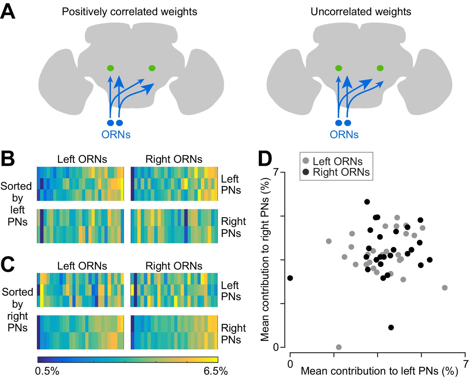
(A) Schematics illustrating alternative scenarios: ORN connection weights may be correlated across PNs or uncorrelated. Arrowhead size represents the strength of ORN→PN connections. ORN spikes faithfully invade both ipsi- and contralateral axonal arbors, and so if connection weights are optimized to reflect the spiking properties of each ORN, then connection weights should be correlated across all ipsi- and contralateral PNs. (B) Contributions of individual ORNs to each PN’s pool of ORN synapses. Values are expressed as the percentage contribution of each ORN to the pool of synapses from that antenna. Within each of these 10 vectors, values sum to 100%. Within an antenna, ORNs are sorted according to the average strength of all the connections that they form onto left PNs. Note that left PNs are correlated with each other, but not with right PNs. (C) Same data as in (B), but now sorted by average strength of connections onto right PNs rather than left PNs. Note that right PNs are correlated with each other, but not with left PNs. When we examined pairs of PNs in the same quadrant, we found that 7 of 8 PN pairs were significantly correlated with each other (Pearson’s r ranges from 0.44 to 0.78, p<0.05, n = 27 or 26 unitary connections for each PN for each test, P values are corrected for multiple comparisons, m = 8 tests). The one exception was that left PN2 and left PN3 were not significantly correlated (Pearson’s r = 0.36, p=0.07 after multiple comparisons correction). When we tested pairs PNs on opposite sides of the midline (again testing separately for correlations among right ORNs and left ORNs), we found that none of the 12 PN pairs were significantly correlated (Pearson’s r ranges from −0.21 to 0.34, P always >0.09, n = 27 or 26 unitary connections for each PN for each test; tests were not corrected for multiple comparisons, as none were significant). (D) Average contribution of each ORN to the PNs on the right side, plotted against the average contribution of the same ORN to the PNs on the left. Percentages are calculated as in (B) before averaging across all the PNs on the same side of the brain. There is no significant correlation (Pearson’s r = 0.18, p=0.20, n = 53 unitary connections for each PN).
Figure 7
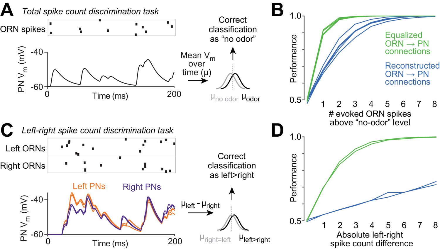
Functional consequences of variability in ORN wiring.
(A) Schematic of 'odor detection’ task. We measured how accurately a binary linear classifier could detect a small increase in ORN spike number, based on the time-averaged voltage in model PNs. Simulated Poisson spike trains were assigned to reconstructed ORN axons and fed into our PN models. Only ORNs ipsilateral to the PN were simulated. Over a 200 ms period, ORNs fired either 12 spikes (the average number of spikes during this time period that DM6 ORNs fire in the absence of an odor), or 13 spikes (representing a minimal odor stimulus). Based on the distribution of the time-averaged PN voltage (µ) in training trials, we classified each test trial as ‘non-odor’ or ‘odor’ (12 or 13 spikes). We repeated this many times for each of the five model PNs. The same procedure was used to measure accuracy when the ‘odor’ elicited increasing numbers of spikes (14 to 20 spikes). (B) Performance of the classifier as a function of the number of ‘odor-evoked’ spikes, above the baseline level of 12 spikes. Each blue line represents a different model PN. As in all previous simulations, the PN dendrite morphology and the locations of all ORN synapses are taken directly from our reconstructions. Green lines show that performance increases after we equalize the number of synapses per connection (by randomly reassigning synapses to ORN axons, so that all axons now have essentially equal numbers of synapses). (C) Schematic of ‘odor lateralization’ task. Here we simulated ‘non-odor’ activity (12 spikes) in one antenna and ‘odor’ activity (13–20 spikes) in the other antenna. Classification was based on the difference between PN voltage values on the left and right (cell-averaged µleft – cell-averaged µright). (D) Performance of the classifier as a function of the number of ‘odor-evoked’ spikes (the left-right asymmetry). The two blue lines represent an odor stimulus in either the right antenna or the left antenna. Green lines show that performance increases after we equalize the number of synapses per connection.
Videos
Video 1
EM volume of the anterior fly brain.
The video shows a fly-through (posterior to anterior) of the aligned EM series. Please see Data Availability for directions to the publicly accessible high-resolution aligned data set.
Video 2
Serial EM sections through left glomerulus DM6.
The video shows a fly-through (anterior to posterior) of a cropped (16.4 µm × 16.4 µm) volume traversing 329 of the aligned EM sections containing glomerulus DM6 neuropil in the left hemisphere of the brain.
Download links
A two-part list of links to download the article, or parts of the article, in various formats.
Downloads (link to download the article as PDF)
Open citations (links to open the citations from this article in various online reference manager services)
Cite this article (links to download the citations from this article in formats compatible with various reference manager tools)
Wiring variations that enable and constrain neural computation in a sensory microcircuit
eLife 6:e24838.
https://doi.org/10.7554/eLife.24838


