Figures and data in Lotka-Volterra pairwise modeling fails to capture diverse pairwise microbial interactions | eLife

Version of Record

Accepted for publication after peer review and revision.

Download
Cite
Share
CommentOpen annotations (there are currently 0 annotations on this page).

Version of Record published: June 13, 2017 (This version)
Accepted Manuscript updated: April 3, 2017 (Go to version)
Accepted Manuscript published: March 28, 2017 (Go to version)
Accepted: March 18, 2017
Received: January 11, 2017

Figures
Additional files

8 figures and 16 additional files

Figures

Figure 1 with 2 supplements

Download asset Open asset

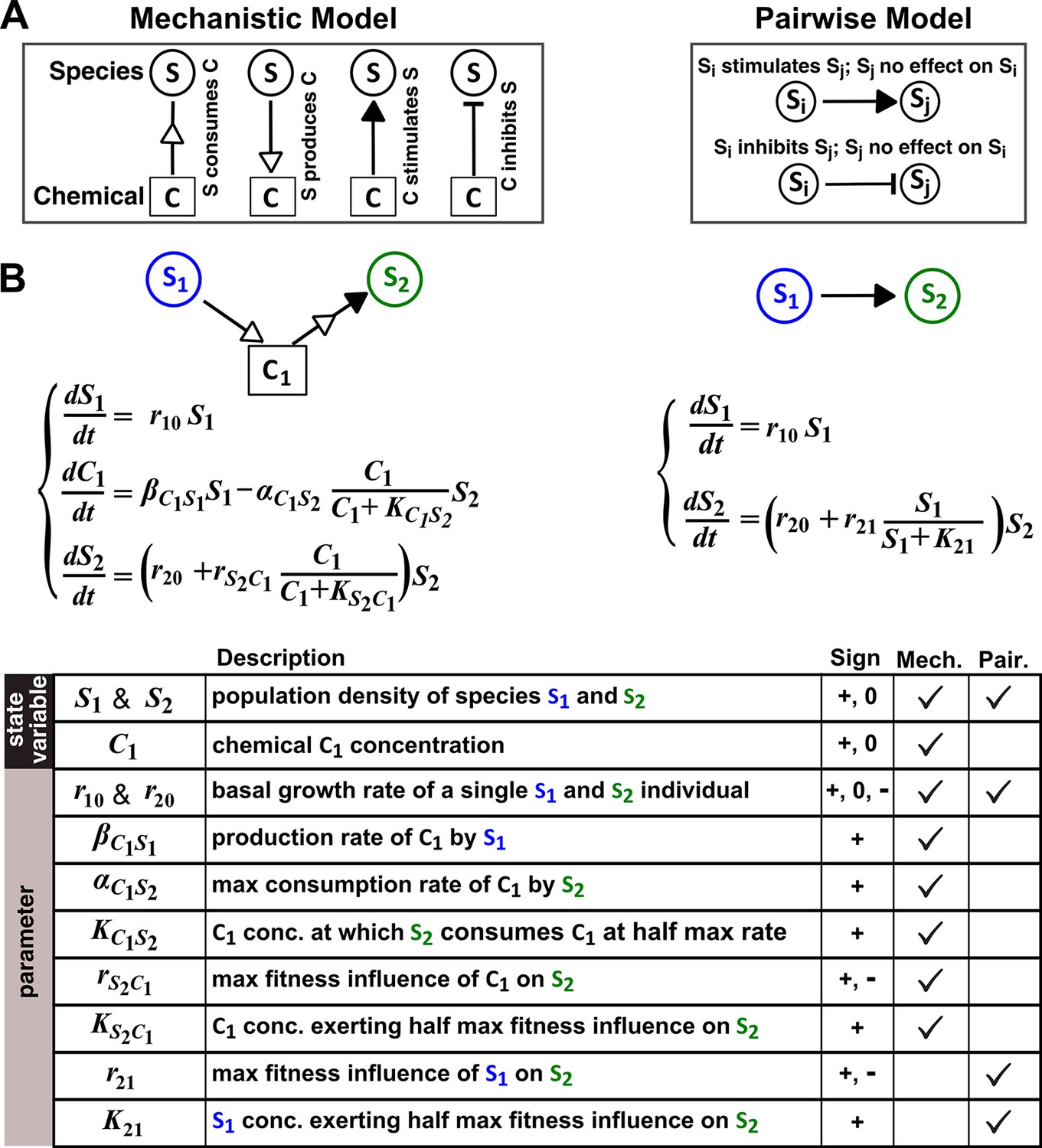
The abstraction of interaction mechanisms in a pairwise model compared to a mechanistic model.

(A) The mechanistic model (left) considers a bipartite network of species and chemical interaction mediators. A species can produce or consume chemicals (open arrowheads pointing towards and away from the chemical, respectively). A chemical mediator can positively or negatively influence the fitness of its target species (filled arrowhead and bar, respectively). The corresponding L-V pairwise model (right) includes only the fitness effects of species interactions, which can be positive (filled arrowhead), negative (bar), or zero (line terminus). (B) In the example here, species S₁ releases chemical C₁, and C₁ is consumed by species S₂ and promotes S₂’s fitness. In the mechanistic model, the three equations respectively state that (1) S₁ grows exponentially at a rate $r_{10}$ , (2) C₁ is released by S₁ at a rate $β_{C_{1} S_{1}}$ and consumed by S₂ with saturable kinetics (maximal consumption rate $α_{C_{1} S_{2}}$ and half-saturation constant $K_{C_{1} S_{2}}$ ), and (3) S₂’s growth (basal fitness $r_{20}$ ) is influenced by C₁ in a saturable fashion. In the pairwise model here, the first equation is identical to that of the mechanistic model. The second equation is similar to the last equation of the mechanistic model except that $r_{21}$ and $K_{21}$ together reflect how the density of S₁ ( $S_{1}$ ) affects the fitness of S₂ in a saturable fashion. For all parameters with double subscripts, the first subscript denotes the focal species or chemical, and the second subscript denotes the influencer. Note that unlike in mechanistic models, we have omitted ‘ $S$ ’ from subscripts in pairwise models (e.g. $r_{21}$ instead of $r_{S_{2} S_{1}}$ ) for simplicity. In this example, both $r_{21}$ and $r_{S_{2} S_{1}}$ are positive.

https://doi.org/10.7554/eLife.25051.003

Figure 1—figure supplement 1

Download asset Open asset

An L-V pairwise model successfully predicts oscillations in population dynamics of the hare-lynx prey-predator community.

(A) In a pairwise model of prey-predation proposed by Lotka and Volterra, predator reduces the fitness of prey, while prey stimulates the fitness of predator. Such dynamics can be easily simulated (Green and Shou, 2014). (B) Assuming random encounter between prey and predator, the pairwise model predicts oscillations in the prey and predator population sizes. (C) Similar oscillations have been qualitatively observed in natural populations of lynx (predator) and hare (prey), providing support for the usefulness of pairwise models. Picture is adapted from https://biologyeoc.wikispaces.com/PopulationChanges (BiologyEOC, 2016).

https://doi.org/10.7554/eLife.25051.004

Figure 1—figure supplement 2

Download asset Open asset

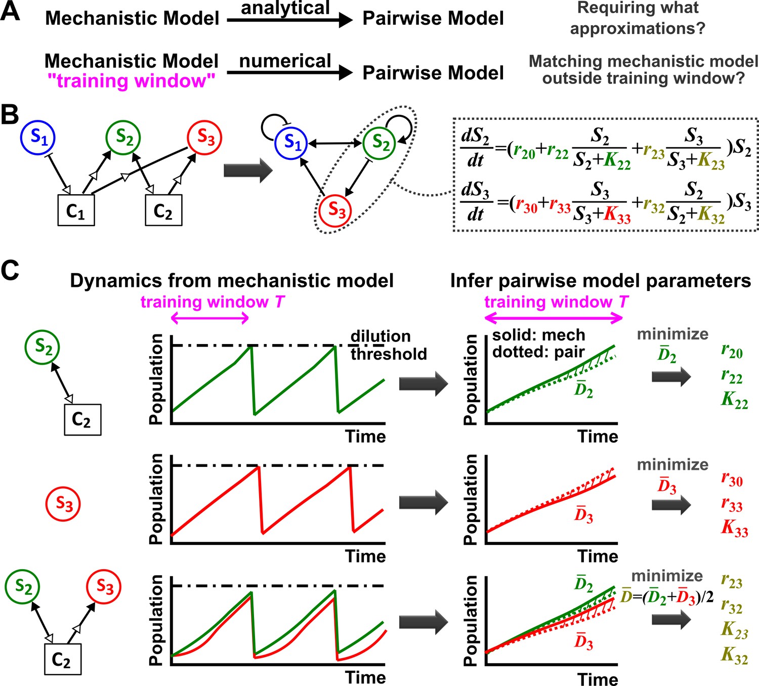
Deriving a pairwise model.

(A) Analytically deriving a pairwise model from a mechanistic model allows us to uncover approximations required for such a transformation (top). Alternatively (bottom), within a ‘training window’ of the mechanistic model population dynamics, we can numerically derive parameters for a pre-selected pairwise model such that it best fits the mechanistic model. We then quantify how well such a pairwise model matches the mechanistic model under conditions different from those of the training window. (B) A mechanistic model of three species interacting via two chemicals (left) can be translated into a pairwise model of three interacting species (center). S₁ inhibits S₁ and promotes S₂ (via C₁). S₂ promotes S₂ and S₃ (via C₂) as well as S₁ (via removal of C₁). S₃ promotes S₁ (via removal of C₁) and inhibits S₂ (via removal of C₂). Take interactions between S₂ and S₃ for example: the saturable L-V pairwise model will require estimating ten parameters (colored, right), some of which (e.g. $r_{33}$ in this case) may be zero. (C) In the numerical method, the six monoculture parameters ( $r_{i 0}$ , $r_{i i}$ , and $K_{i i}$ , $i$ = 2, 3; green and red) are first estimated from training window $T$ (within a dilution cycle) of monoculture mechanistic models (top and middle). Subsequently, the four interaction parameters ( and $K_{i j}$ , , olive) can be estimated from the training window $T$ of the S₂ +S₃ coculture mechanistic model (bottom). Parameter definitions are described in Figure 1. Often in this work, pairwise model parameters that can be directly obtained from the mechanistic model (e.g. species basal fitness; ) are directly obtained from the mechanistic model (instead of being estimated). To estimate parameters, we use an optimization routine to minimize $\bar{D}$ , the fold-difference (hatched area) between dynamics from a pairwise model (dotted lines) and the mechanistic model (solid lines) averaged over $T$ and species number $N$ : $\bar{D} = \frac{1}{N} \sum_{i = 1}^{N} [\frac{1}{T} \int_{T} D_{i} (t) d t] = \frac{1}{N} \sum_{i = 1}^{N} [\frac{1}{T} \int_{T} | l o g_{10} (S_{i, p a i r} (t) / S_{i, m e c h} (t)) | d t]$ . Here $S_{i, p a i r}$ and $S_{i, m e c h}$ are $S_{i}$ calculated using pairwise and mechanistic models, respectively. Since species with densities below a set extinction limit, $S_{e x t}$ , are assumed to have gone extinct in the model, we set all densities below the extinction limit to $S_{e x t}$ in calculating $\bar{D}$ to avoid singularities. $\bar{D}$ outside the training window can be used to quantify how well the best-matching pairwise model predicts the mechanistic model. Unless otherwise stated, in all simulations to ensure that resources not involved in interactions are never limiting, a community is diluted back to its inoculation density whenever total population increases to a high-density threshold, mimicking turbidostat experiments. Too frequent dilutions will allow only small changes in population dynamics within a dilution cycle or time $T$ , which is not suitable for estimating pairwise model parameters. Dilutions can sometimes violate conditions for convergence to reference dynamics (Figure 3—figure supplement 4). Under most cases we have tested, small variations in dilution frequency do not affect our conclusions. See Methods-Summary of simulation files for relevant Matlab codes.

https://doi.org/10.7554/eLife.25051.005

Figure 2

Download asset Open asset

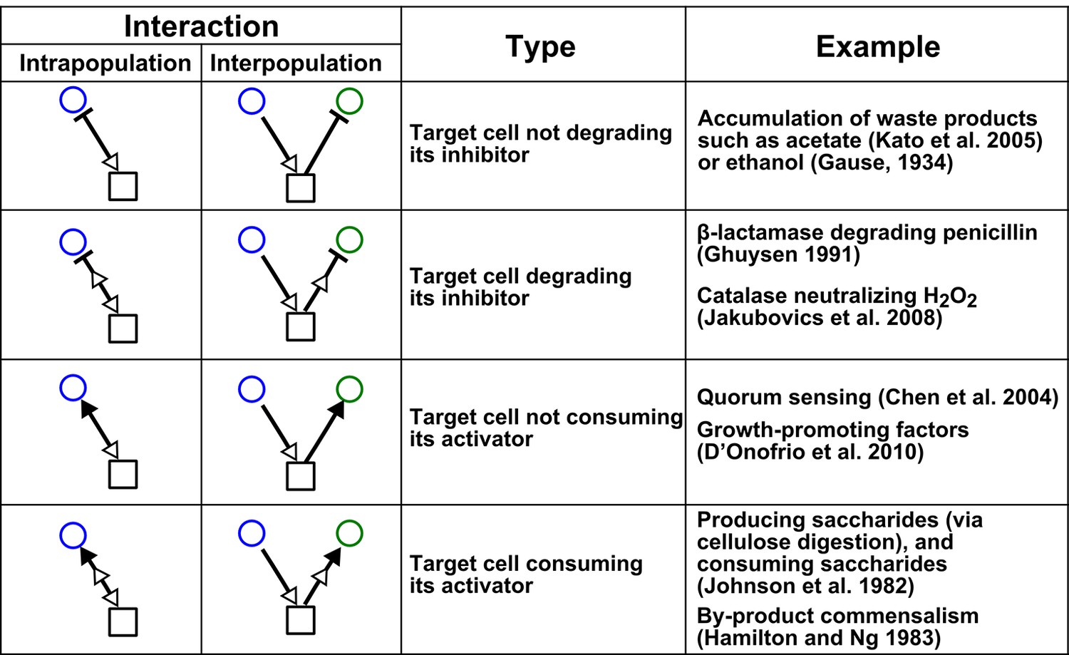
Chemical-mediated interactions commonly found in microbial communities.

Interactions can be intra- or inter-population. Examples are meant to be illustrative instead of comprehensive.

https://doi.org/10.7554/eLife.25051.006

Figure 3 with 5 supplements

Download asset Open asset

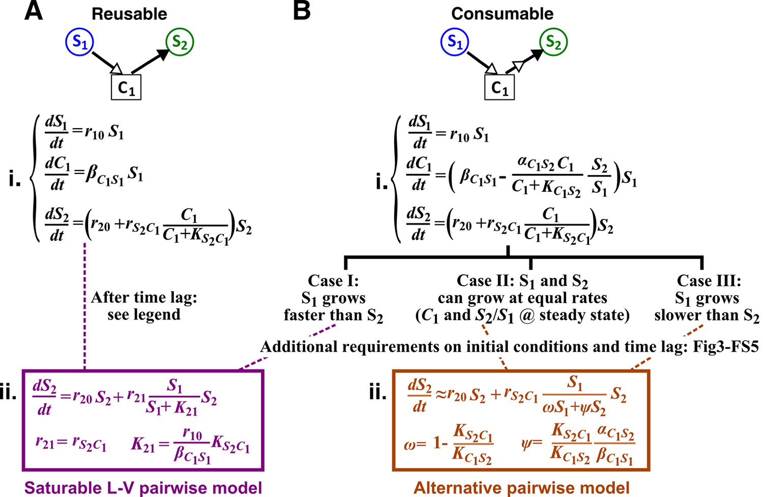
Interactions mediated via a single mediator are best represented by different forms of pairwise models, depending on whether the mediator is consumable or reusable and on the relative fitness and initial densities of the two species.

S₁ stimulates the growth of S₂ via a reusable (A) or a consumable (B) chemical C₁. In mechanistic models of the two cases (i), equations for $S_{1}$ and $S_{2}$ are identical but equations for $C_{1}$ are different. In (A), $C_{1}$ can be solved to yield $C_{1} = (β_{C_{1} S_{1}} / r_{10}) S_{10} \exp (r_{10} t) - (β_{C_{1} S_{1}} / r_{10}) S_{10} = (β_{C_{1} S_{1}} / r_{10}) S_{1} - (β_{C_{1} S_{1}} / r_{10}) S_{10}$ , assuming zero initial $C_{1}$ . Here, $S_{10}$ is $S_{1}$ at time zero. We have approximated $C_{1}$ by omitting the second term (valid after the initial transient response has passed so that $C_{1}$ has become proportional to $S_{1}$ ). This approximation allows an exact match between the mechanistic model and the saturable L-V pairwise model (ii). In (B), depending on the relative growth rates of the two species, and if additional requirements are satisfied (Methods; Figure 3—figure supplement 2; Figure 3—figure supplement 3; Figure 3—figure supplement 4; Figure 3—figure supplement 5), either saturable L-V or alternative pairwise model should be used.

https://doi.org/10.7554/eLife.25051.007

Figure 3—source data 1 List of parameters for simulations in Figure 3—figure supplement 1.: https://doi.org/10.7554/eLife.25051.008
Download elife-25051-fig3-data1-v3.docx
Figure 3—source data 2 List of parameters for simulations in Figure 3—figure supplement 2 on interactions through a consumable mediator.: https://doi.org/10.7554/eLife.25051.009
Download elife-25051-fig3-data2-v3.docx
Figure 3—source data 3 List of parameters for simulations in Figure 3—figure supplement 3 on conditions required for convergence of the alternative pairwise model.: https://doi.org/10.7554/eLife.25051.010
Download elife-25051-fig3-data3-v3.docx
Figure 3—source data 4 List of parameters for simulations in Figure 3—figure supplement 4 on how dilution might affect the convergence of a pairwise model.: https://doi.org/10.7554/eLife.25051.011
Download elife-25051-fig3-data4-v3.docx

Figure 3—figure supplement 1

Download asset Open asset

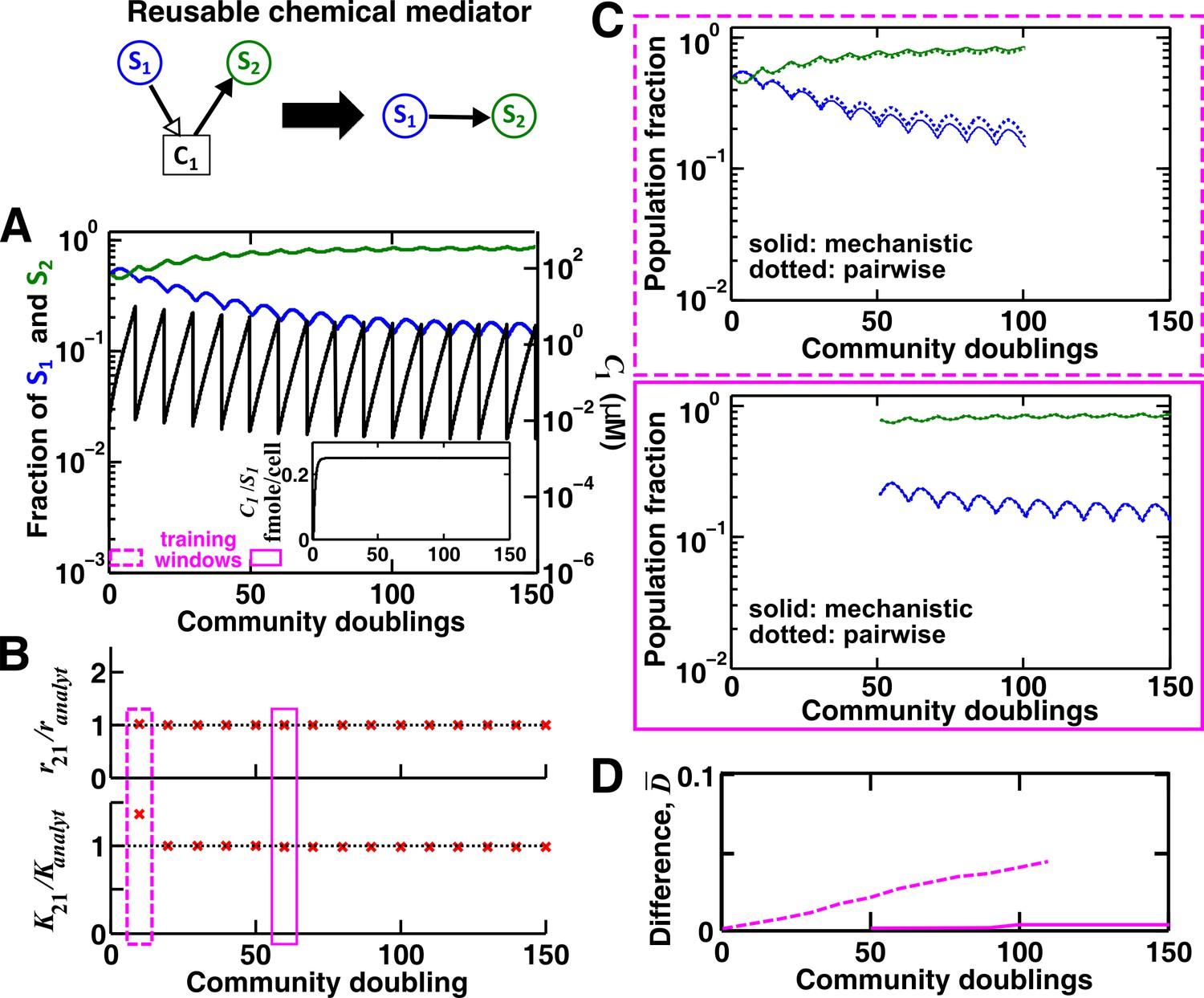
For a reusable mediator, parameter estimation after acclimation time leads to a more accurate saturable L-V pairwise model.

(A) We use the mechanistic model for a reusable mediator to generate reference dynamics of , , and over 150 generations of community growth. Note that population fractions (instead of population densities) are plotted, which fluctuate less than the mediator concentration during dilutions. After an initial period of time, becomes proportional to (inset). The basal fitness of S₁ and S₂ in pairwise models are identical to those in mechanistic models, and here and (= 1, 2) are irrelevant due to the lack of intra-population interactions. We use every 10 community doublings (within a dilution cycle) of reference dynamics as training windows to numerically estimate best-matching saturable L-V pairwise model parameters and . Dashed and solid rectangles represent a training window before and after acclimation, respectively. (B) Pairwise model parameters estimated after acclimation (e.g. solid rectangle) match their analytically-derived counterparts (black dotted lines) better than those estimated before acclimation (e.g. dashed rectangle). (C) A pairwise model generated from population dynamics before acclimation (top) predicts future reference dynamics less accurately than that generated after acclimation (bottom). (D) Quantification of the difference between pairwise and mechanistic models before (dashed) or after (solid) acclimation. All parameters are listed in Figure 3—source data 1.

https://doi.org/10.7554/eLife.25051.012

Figure 3—figure supplement 2

Download asset Open asset

Community trajectory approaching the -zero-isocline allows us to use the alternative pairwise model approximation.

S₁ releases a consumable metabolite C₁ which stimulates S₂ growth. In all panels, brown circles indicate the $C_{1}$ and $R_{S}$ ( $= S_{2} / S_{1}$ ) of a community, and are separated by 1/4 of community doubling time. In the vicinity of the $f$ -zero-isocline ( $f = 0$ ) (blue line), can be eliminated to yield a pairwise model. (A–D) When $r_{S_{2} C_{1}} > r_{10} - r_{20} > 0$ (Methods-Deriving a pairwise model for interactions mediated by a single consumable mediator, Case II), a steady state (green circle) exists. Let us scale and against their respective steady state values to obtain ${\hat{R}}_{S}$ and ${\hat{C}}_{1}$ . The $f$ -zero-isocline (blue) and the steady state ${\hat{C}}_{1} = 1$ (vertical solid line) divide the phase portrait into four regions (① to ④). (A) The directions of movement are marked by grey arrowheads. According to the top portion of Equation 11,the right-hand side of Equation 14 is zero when ${\hat{C}}_{1} = 1$ . Since ${\hat{C}}_{1} / ({\hat{C}}_{1} + {\hat{K}}_{S_{2} C_{1}}) = 1 / (1 + {\hat{K}}_{S_{2} C_{1}} / {\hat{C}}_{1})$ is an increasing function of ${\hat{C}}_{1}$ , when ${\hat{C}}_{1} > 1$ , $d {\hat{R}}_{S} / d t$ > 0 (up arrows), and when ${\hat{C}}_{1}$ <1, $d {\hat{R}}_{S} / d t$ <0 (down arrows). From Equation 15, above the $f$ -zero-isocline, $d {\hat{C}}_{1} / d t$ <0 (left arrows), while below the $f$ -zero-isocline, $d {\hat{C}}_{1} / d t$ >0 (right arrows). Thus, the community moves toward the $f$ -zero-isocline, and then moves slowly alongside (but not superimposing) the $f$ -zero-isocline before reaching the steady state. A–C respectively describe community dynamics trajectories from when $S_{10}$ is large and when ${\hat{R}}_{S} (t = 0) \approx 1$ (Case II-2), ${\hat{R}}_{S} (t = 0) ≫ max (1, {\hat{K}}_{S_{2} C_{1}}^{- 1})$ (Case II-1), or ${\hat{R}}_{S} (t = 0) ≪ 1 / (1 + {\hat{K}}_{C_{1} S_{2}})$ (Case II-3). (D) ${\hat{R}}_{S} (t = 0) \approx 1$ but $S_{10}$ is much smaller than that in A. In this case, instead of approaching the $f$ -zero-isocline quickly as in A, the trajectory plunges sharply before moving toward the $f$ -zero-isocline. The black dotted line marks ${\hat{R}}_{S} = 1 / (1 + {\hat{K}}_{C_{1} S_{2}})$ , the asymptotic value of $f$ -zero-isocline. (E–H) When $r_{10} - r_{20} < 0$ (Methods-Deriving a pairwise model for interactions mediated by a single consumable mediator, Case III), there is no steady state. $R_{S}$ approaches infinity and $C_{1}$ approaches 0. The black dotted line marks $R_{S} = β_{C_{1} S_{1}} / α_{C_{1} S_{2}}$ , the asymptotic value of $f$ -zero-isocline. E, F, and G respectively describe community dynamics trajectories from $C_{1} = 0$ when $S_{10}$ is large and when $R_{S} (0) \approx β_{C_{1} S_{1}} / α_{C_{1} S_{2}}$ , $R_{S} (0) ≫ β_{C_{1} S_{1}} / α_{C_{1} S_{2}}$ (Case III-1), and $R_{S} (0) ≪ β_{C_{1} S_{1}} / α_{C_{1} S_{2}}$ (Case III-2). (H) $R_{S} (0) ≫ β_{C_{1} S_{1}} / α_{C_{1} S_{2}}$ but $S_{10}$ is much smaller than that in F. Note different axis scales in different figure panels. All parameters are listed in Figure 3—source data 2.

https://doi.org/10.7554/eLife.25051.013

Figure 3—figure supplement 3

Download asset Open asset

Condition for the alternative pairwise model to converge to the mechanistic model in the absence of dilutions.

Here are the phase portraits of Equation 43. The olive vertical dotted lines correspond to $R_{S} = - ω / ψ$ , a singularity point when $ω < 0$ . (A) Case II ( $r_{S_{2} C_{1}} > r_{10} - r_{20} > 0$ ), $ω = 0.5$ , $ψ = 0.25$ . Regardless of initial , the solution converges to steady state (in agreement with the mechanistic model). (B) Case II, $ω = - 1$ , $ψ = 1$ . When $R_{S} (t = 0) < - ω / ψ$ (to the left of olive line), the alternative pairwise model falsely predicts extinction of S₂. (C) Case III ( $r_{10} < r_{20}$ ), $ω = 0.8$ , $ψ = 0.1$ . Regardless of initial , the model predicts extinction of S₁ (in agreement with the mechanistic model). (D) Case III ( $r_{10} < r_{20}$ ), $ω = - 9$ , $ψ = 5$ . When $R_{S} (t = 0) < - ω / ψ$ (to the left of olive line), the alternative pairwise model falsely predicts steady state coexistence of the two species. All parameters are listed in Figure 3—source data 3.

https://doi.org/10.7554/eLife.25051.014

Figure 3—figure supplement 4

Download asset Open asset

Initial conditions that require long convergence time and thus dilutions may prevent the alternative pairwise model to converge to the mechanistic model.

We consider commensalism through a consumable mediator, where the producer and the consumer could reach a steady state (Methods-Deriving a pairwise model for interactions mediated by a single consumable mediator, Case II). We choose a low consumption rate such that starting from equal proportions of producers and consumers, consumption can be neglected. (A) When the initial total population density is low (2 × 10⁵ total cells/ml, and periodic 10x dilution maintains this low density), the community cannot approach the blue -zero-isocline in a reasonable time frame (brown trajectory in the phase space of ${\hat{C}}_{1}$ and ${\hat{R}}_{S}$ , the mediator concentration and the consumer-to-producer ratio normalized to their potential steady state values, respectively). As a result, growth and dilution lead to an alternate sustained cycle for the community (inset). (B) In this case, accumulates proportionally to within each dilution cycle, and the ratio of to reaches a constant value (inset). (C) Since behaves as a reusable mediator and since the community remains far from the -zero-isocline, the use of the alternative pairwise model (dashed) is not justified. Instead, the saturable L-V pairwise model (dotted) provides a better approximation. (D) The same community at a higher initial total density (2 × 10⁸ total cells/ml) approaches the blue -zero-isocline (brown trajectory in the phase space) after a few dilutions. (E) In the vicinity of the -zero-isocline, reaches its steady state value within each dilution cycle. (F) In this case, the alternative model produces a better approximation to the mechanistic model compared to a saturable L-V model. In (C) and (F), the saturable L-V model is fitted into dynamics of the reference model after 50 generations, whereas analytical formulas are used for the alternative pairwise model. All parameters are listed in Figure 3—source data 4.

https://doi.org/10.7554/eLife.25051.015

Figure 3—figure supplement 5

Download asset Open asset

Additional requirements for deriving a pairwise model from a mechanistic model, when S₁ affects S₂ via a single consumable mediator C₁ where $C_{1} (0) = 0$ .

For details, see Methods. Here, $R_{S} = S_{2} / S_{1}$ . $S_{1} (0)$ , $S_{2} (0)$ , $C_{1} (0)$ , and $R_{S} (0)$ are the initial values of the respective variables. (A) The initial condition requirement for a pairwise model to converge to the mechanistic model. (B) The time scale required for convergence. Conditions on $S_{1} (0)$ are sufficient, but may not be necessary.

https://doi.org/10.7554/eLife.25051.016

Figure 4

Download asset Open asset

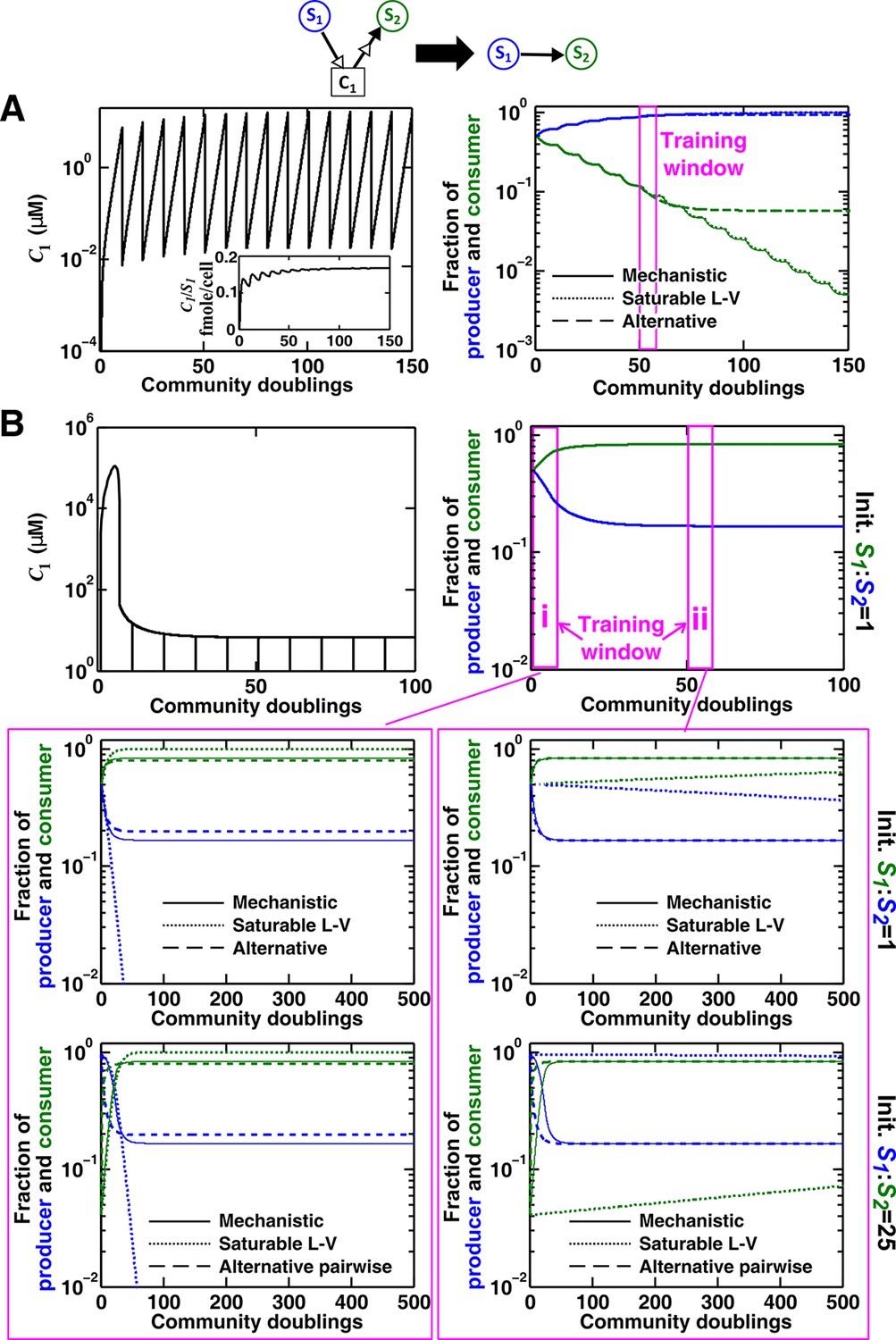
Saturable L-V and alternative pairwise models are not interchangeable.

Consider a commensal community with a consumable mediator C₁. (A) The mediator accumulates without reaching a steady state within each dilution cycle as the consumer S₂ gradually goes extinct (Figure 3B, Case I). After a few tens of generations, $C_{1}$ becomes proportional to its producer density $S_{1}$ (inset in left panel). In this case, a saturable L-V (dotted) but not the alternative pairwise model (dashed) is suitable. All parameters are listed in Figure 4—source data 1. (B) The consumable mediator reaches a non-zero steady state within each dilution cycle (Figure 3B, Case II). From mechanistic dynamics where initial species ratio is 1, we use two training windows to derive saturable L-V (dotted) and alternative (dashed) pairwise models. We then use these pairwise models to predict dynamics of communities starting at two different ratios. The alternative model but not the saturable L-V predicts the mechanistic model dynamics. All parameters are listed in Figure 4—source data 2. Note that in all figures, population fractions (instead of population densities) are plotted, which fluctuate less during dilutions compared to mediator concentration.

https://doi.org/10.7554/eLife.25051.017

Figure 4—source data 1 List of parameters for simulations in Figure 4 on an interaction through a reusable mediator.: https://doi.org/10.7554/eLife.25051.018
Download elife-25051-fig4-data1-v3.docx
Figure 4—source data 2 List of parameters for simulations in Figure 4 on an interaction through a consumable mediator.: https://doi.org/10.7554/eLife.25051.019
Download elife-25051-fig4-data2-v3.docx

Figure 5 with 1 supplement

Download asset Open asset

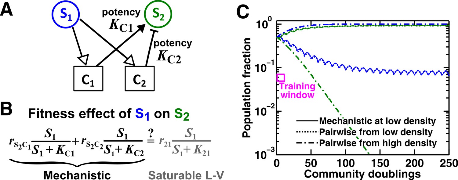
An example of a two-mediator interaction where a saturable L-V pairwise model may succeed or fail depending on initial conditions.

(A) One species can affect another species via two reusable mediators, each with a different potency $K_{C i}$ where $K_{C i}$ is $K_{S_{2} C_{i}} r_{10} / β_{C_{i} S_{1}}$ (Methods-Conditions under which a saturable L-V pairwise model can represent one species influencing another via two reusable mediators). A low $K_{C i}$ indicates a strong potency (e.g. high release of C_i by S₁ or low $C_{i}$ required to achieve half-maximal influence on S₂). (B) Under what conditions can an interaction via two reusable mediators with saturable effects on recipients be approximated by a saturable L-V pairwise model? (C) A community where the success or failure of a saturable L-V pairwise model depends on initial conditions. Here, $K_{C 1}$ = 10³ cells/ml and $K_{C 2}$ = 10⁵ cells/ml. Community dynamics starting at low $S_{1}$ (solid) can be predicted if the saturable L-V pairwise model is derived from reference dynamics starting at low (dotted). However, if we use a saturable L-V pairwise model derived from a community with high initial $S_{1}$ , prediction is qualitatively wrong (dash dot line). See Figure 5—figure supplement 1D for an explanation why a saturable L-V pairwise model estimated at one community density may not be applicable to another community density. Simulation parameters are listed in Figure 5—source data 1 .

https://doi.org/10.7554/eLife.25051.020

Figure 5—source data 1 List of parameters for simulations in Figure 5 on an interaction through two concurrent mediators.: https://doi.org/10.7554/eLife.25051.021
Download elife-25051-fig5-data1-v3.docx
Figure 5—source data 2 List of parameters for simulations in Figure 5—figure supplement 1 on an interaction through two concurrent mediators, assessed at high versus low cell densities.: https://doi.org/10.7554/eLife.25051.022
Download elife-25051-fig5-data2-v3.docx

Figure 5—figure supplement 1

Download asset Open asset

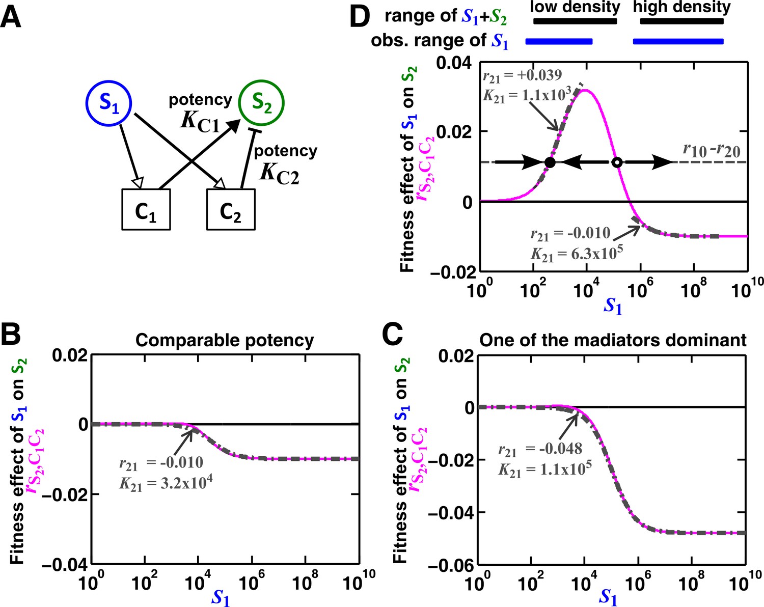
Except under special conditions, a pairwise interaction through two mediators may not be represented by a single saturable L-V model.

(A) Consider the interaction in Figure 5. The fitness effect of S₁ on S₂ via C₁ and C₂ is $r_{S_{2}, C_{1} C_{2}} = \frac{r_{S_{2} C_{1}} S_{1}}{S_{1} + K_{S_{2} C_{1}} r_{10} / β_{C_{1} S_{1}}} + \frac{r_{S_{2} C_{2}} S_{1}}{S_{1} + K_{S_{2} C_{2}} r_{10} / β_{C_{2} S_{1}}} = \frac{r_{S_{2} C_{1}} S_{1}}{S_{1} + K_{C_{1}}} + \frac{r_{S_{2} C_{2}} S_{1}}{S_{1} + K_{C_{2}}}$ . (B–C) Under special conditions the fitness effect $r_{S_{2}, C_{1} C_{2}}$ (magenta line) can be approximated using a single saturable L-V model (grey dash-dot line) at all densities. These special conditions include when the potencies of two mediators, K_C1 and K_C2, are similar (B) or the potency of one mediator is orders of magnitude stronger than the other (C). Otherwise, saturable L-V pairwise models derived from a low-density community and from a high-density community can have qualitatively different parameters (D). Let’s first consider the low-density case (left black and blue bars corresponding to low total density and therefore low , respectively). When $r_{S_{2}, C_{1} C_{2}}$ (magenta line) is above the ( $r_{10} - r_{20}$ ) line (grey dashed line), the fitness of S₂ ( $r_{S_{2}, C_{1} C_{2}} + r_{20}$ ) will be higher than the fitness of S₁. Thus, even though S₁ grows at its basal fitness during a dilution cycle, S₁ fraction will decrease. Thus $S_{1}$ will decrease at the next dilution cycle when total density is reset to a pre-fixed level (arrow pointing towards lower $S_{1}$ ). In contrast, when $r_{S_{2}, C_{1} C_{2}} < r_{10} - r_{20}$ , S₁ population fraction and $S_{1}$ will increase at the next dilution cycle (arrow pointing towards higher $S_{1}$ ). Thus, the dynamics will converge to a steady state ratio (filled dot). Interaction coefficient of a saturable L-V (grey dash-dot line) is estimated to be a positive value ( =+0.039). In contrast, in the high-density case (right black and blue bars), $r_{10} > r_{S_{2}, C_{1} C_{2}} + r_{20}$ , and S₂ goes extinct. Interaction coefficient of a saturable L-V (grey dash-dot line) is estimated to be a negative value ( = −0.010). As a result, a saturable L-V pairwise model with parameters estimated at high densities cannot predict communities at low densities (Figure 5). All parameters are listed in Figure 5—source data 2.

https://doi.org/10.7554/eLife.25051.023

Figure 6

Download asset Open asset

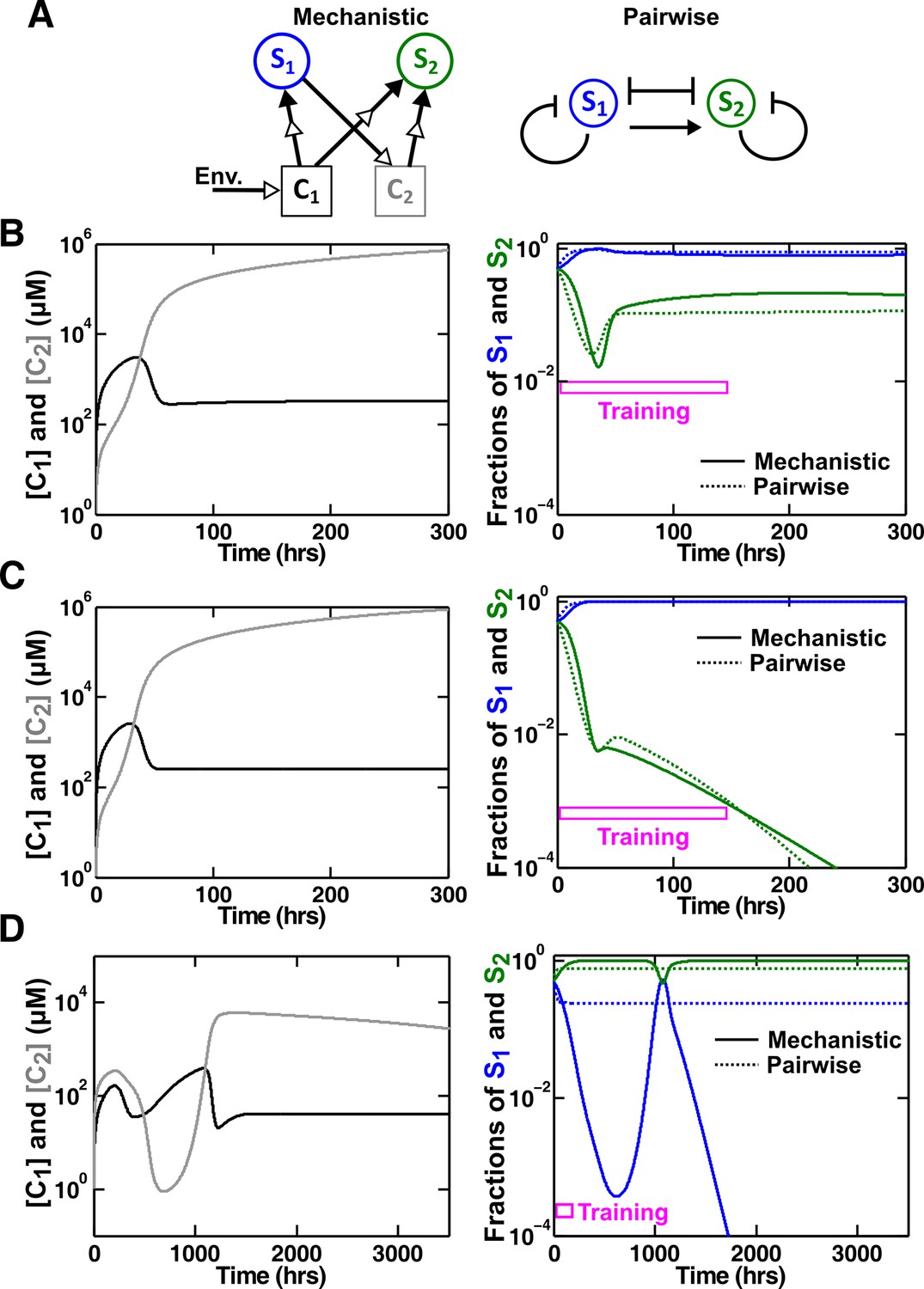
An example of a competitive commensal community where an L-V pairwise model may work or fail.

(A) Left: Two species S₁ and S₂ compete for shared resource C₁. Additionally, S₁ produces C₂ that promotes the growth of S₂ upon consumption. Right: An L-V pairwise model captures the intra- and inter-species competition as well as the commensal interaction between the two species. (B,C) Examples where L-V pairwise models predict the mechanistic reference dynamics well. (D) An example where the L-V pairwise model fails to predict the dynamics qualitatively (note the much longer time range). Here, population fractions fluctuate due to changes in relative concentration of C₁ compared to C₂. In all cases, the pairwise model is derived from the population dynamics in the initial stages of growth (150 hr in all cases). Simulation parameters are listed in Figure 6—source data 1.

https://doi.org/10.7554/eLife.25051.024

Figure 6—source data 1 List of parameters for simulations in Figure 6 on an interaction through a consumable mediator, for species consuming a shared abiotic resource.: https://doi.org/10.7554/eLife.25051.025
Download elife-25051-fig6-data1-v3.docx

Figure 7 with 1 supplement

Download asset Open asset

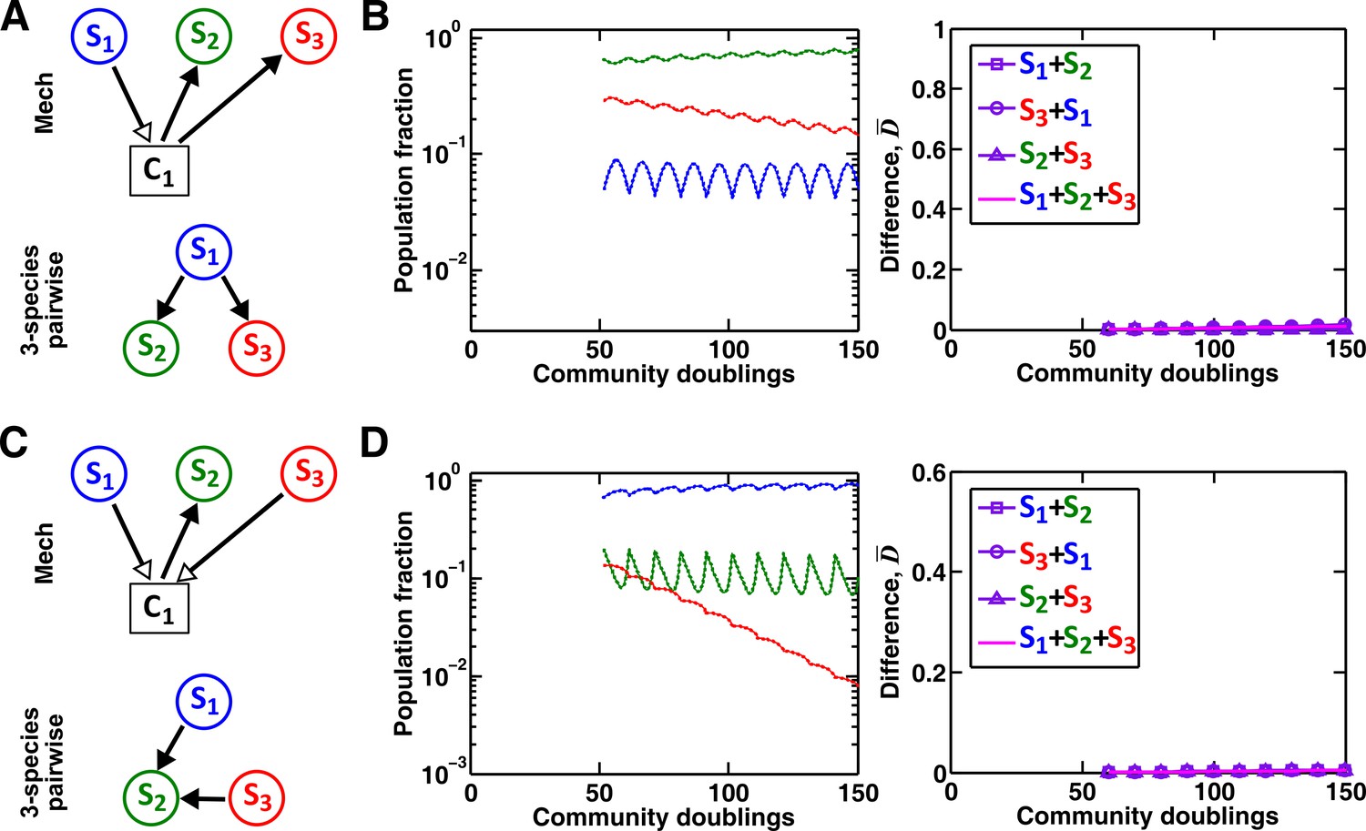
Interaction chain but not interaction modification may be represented by a multispecies pairwise model.

We examine three-species communities engaging in indirect interactions. Each species pair is representable by a two-species pairwise model (saturable L-V or alternative pairwise model, purple in the right columns of B, D, and F). We then use these two-species pairwise models to construct a three-species pairwise model, and test how well it predicts the dynamics known from the mechanistic model. In B, D, and F, left panels show dynamics from the mechanistic models (solid lines) and three-species pairwise models (dotted lines). Right panels show the difference metric $\bar{D}$ . (A–B) Interaction chain: S₁ affects S₂, and S₂ affects S₃. The two interactions employ independent mediators C₁ and C₂, and both interactions can be represented by the saturable L-V pairwise model. The three-species pairwise model matches the mechanistic model in this case. Simulation parameters are provided in Figure 7—source data 1. (C–F) Interaction modification. In both cases, the three-species pairwise model fails to predict reference dynamics even though the dynamics of each species pair can be represented by a pairwise model. (C–D) S₃ consumes C₁, a mediator by which S₁ stimulates S₂. Parameters are listed in Figure 7—source data 2. Here, S₁ changes the nature of interaction between S₂ and S₃: S₂ and S₃ do not interact in the absence of S₁, but S₃ inhibits S₂ in the presence of S₁. The three-species pairwise model makes qualitatively wrong prediction about species coexistence. As expected, if S₃ does not remove C₁, the three-species pairwise model works (Figure 7—figure supplement 1A–B). (E–F) S₁ and S₃ both supply C₁ which stimulates S₂. Here, no species changes ‘the nature of interactions’ between any other two species: both S₁ and S₃ contribute reusable C₁ to stimulate S₂. S₁ promotes S₂ regardless of S₃; S₃ promotes S₂ regardless of S₁; S₁ and S₃ do not interact regardless of S₂. However, a multispecies pairwise model assumes that the fitness effects from the two producers on S₂ will be additive, whereas in reality, the fitness effect on S₂ saturates at high . As a result, the three-species pairwise model qualitatively fails to capture relative species abundance. As expected, if C₁ affects S₂ in a linear fashion, the community dynamics is accurately captured in the multispecies pairwise model (Figure 7—figure supplement 1C–D). Simulation parameters are listed in Figure 7—source data 3.

https://doi.org/10.7554/eLife.25051.026

Figure 7—source data 1 List of parameters for simulations in Figure 7B on interaction between three species in a chain.: https://doi.org/10.7554/eLife.25051.027
Download elife-25051-fig7-data1-v3.docx
Figure 7—source data 2 List of parameters for simulations in Figure 7D on interaction modification through consumption of a shared mediator by a third species.: https://doi.org/10.7554/eLife.25051.028
Download elife-25051-fig7-data2-v3.docx
Figure 7—source data 3 List of parameters for simulations in Figure 7F on interaction modification through production of a shared mediator by a third species.: https://doi.org/10.7554/eLife.25051.029
Download elife-25051-fig7-data3-v3.docx
Figure 7—source data 4 List of parameters for simulations in Figure 7—figure supplement 1B on an interaction between three species through a shared reusable mediator affecting multiple species.: https://doi.org/10.7554/eLife.25051.030
Download elife-25051-fig7-data4-v3.docx
Figure 7—source data 5 List of parameters for simulations in Figure 7—figure supplement 1D on an interaction between three species through a shared reusable mediator produced by multiple species.: https://doi.org/10.7554/eLife.25051.031
Download elife-25051-fig7-data5-v3.docx

Figure 7—figure supplement 1

Download asset Open asset

A multispecies pairwise model can work under special conditions.

(A–B) As a control for Figure 7C, if S₃ does not remove the mediator of interaction between S₁ and S₂, a three-species pairwise model accurately matches the mechanistic model. Simulation parameters are provided in Figure 7—source data 4. (C–D) As a control for Figure 7E, we ensured that fitness effects from multiple species are additive. In this case, a three-species pairwise model can represent the mechanistic model. To ensure the linearity and additivity of fitness effects, we have used a larger value of half saturation concentration ( $K_{S_{2} C_{1}}$ =10³ μM, instead of 10⁻¹ μM in Figure 7E–F). We have adjusted the interaction coefficients accordingly such that the overall interaction strength exerted by S₁ and S₃ on S₂ is comparable to that in Figure 7E–F (as evident by comparable population compositions). Since the interaction influences under these conditions remain in the linear range, the three-species pairwise model accurately predicts the reference dynamics. Simulation parameters are provided in Figure 7—source data 5.

https://doi.org/10.7554/eLife.25051.032

Figure 8

Download asset Open asset

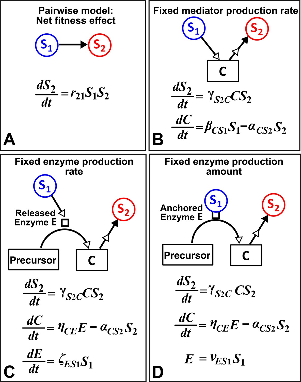
Different levels of abstraction in a mechanistic model.

How one species (S₁) may influence another (S₂) can be mechanistically modeled at different levels of abstraction. For simplicity, here we assume that interaction strength scales in a linear (instead of saturable) fashion with respect to mediator concentration or species density. The basal fitness of S₂ is zero. (A) In the simplest form, S₁ stimulates S₂ in an L-V pairwise model. (B) In a mechanistic model, we may realize that S₁ stimulates S₂ via a mediator C which is consumed by S₂. The corresponding mechanistic model is given. (C) Upon probing more deeply, it may become clear that S₁ stimulates S₂ via an enzyme E, where E degrades an abundant precursor (such as cellulose) to generate mediator C (such as glucose). In the corresponding mechanistic model, we may assume that E is released by S₁ at a rate $ζ_{E S 1}$ and that E liberates C at a rate $η_{C E}$ . (D) If instead E is anchored on the cell surface (e.g. cellulosome), then E is proportional to S₁. If we substitute E into the second equation, then (B) and (D) become equivalent. Thus, when enzyme is anchored on cell surface but not when enzyme is released, the mechanistic knowledge of enzyme can be neglected.

https://doi.org/10.7554/eLife.25051.033

Additional files

Source code 1 Calculates the cost function for monocultures (i.e. the difference between the target mechanistic model dynamics and the dynamics obtained from the pairwise model).: https://doi.org/10.7554/eLife.25051.034
Download elife-25051-code1-v3.m
Source code 2 Calculates the cost function for communities (i.e. the difference between the target mechanistic model dynamics and the dynamics obtained from the saturable L-V pairwise model).: https://doi.org/10.7554/eLife.25051.035
Download elife-25051-code2-v3.m
Source code 3 Calculates the cost function for communities (i.e. the difference between the target mechanistic model dynamics and the dynamics obtained from the alternative pairwise model).: https://doi.org/10.7554/eLife.25051.036
Download elife-25051-code3-v3.m
Source code 4 Returns growth dynamics for monocultures, based on the mechanistic model.: https://doi.org/10.7554/eLife.25051.037
Download elife-25051-code4-v3.m
Source code 5 Returns growth dynamics for communities of multiple species, based on the mechanistic model.: https://doi.org/10.7554/eLife.25051.038
Download elife-25051-code5-v3.m
Source code 6 Returns growth dynamics for communities of multiple species, based on the saturable L-V pairwise model.: https://doi.org/10.7554/eLife.25051.039
Download elife-25051-code6-v3.m
Source code 7 Returns growth dynamics for communities of multiple species, based on the alternative pairwise model.: https://doi.org/10.7554/eLife.25051.040
Download elife-25051-code7-v3.m
Source code 8 Estimates monoculture parameters of pairwise model (Step 1).: https://doi.org/10.7554/eLife.25051.041
Download elife-25051-code8-v3.m
Source code 9 Estimates saturable L-V pairwise model interaction parameters (Step 2).: https://doi.org/10.7554/eLife.25051.042
Download elife-25051-code9-v3.m
Source code 10 Estimates alternative pairwise model interaction parameters (Step 2).: https://doi.org/10.7554/eLife.25051.043
Download elife-25051-code10-v3.m
Source code 11

Estimates saturable L-V pairwise model interaction parameters (r₂₁and K₂₁) in cases where we know that S₂ is only affected by S₁, to accelerate optimization.: https://doi.org/10.7554/eLife.25051.044
Download elife-25051-code11-v3.m
Source code 12

Estimates alternative pairwise model interaction parameter (r₂₁) in cases where we know that S₂ is only affected by S₁ and that K_S2C1=K_C1S2 to accelerate optimization.: https://doi.org/10.7554/eLife.25051.045
Download elife-25051-code12-v3.m
Source code 13 Returns growth dynamics for communities of two species competing for an environmental resource while engaging in an additional interaction, based on the logistic L-V pairwise model (Figure 6).: https://doi.org/10.7554/eLife.25051.046
Download elife-25051-code13-v3.m
Source code 14 Estimates logistic L-V pairwise model interaction parameters for communities of two species competing for an environmental resource while engaging in an additional interaction, and compares community dynamics from pairwise and mechanistic models (Figure 6).: https://doi.org/10.7554/eLife.25051.047
Download elife-25051-code14-v3.m
Source code 15 Defines differential equations when using Matlab’s ODE23 solver to calculate community dynamics.: https://doi.org/10.7554/eLife.25051.048
Download elife-25051-code15-v3.m
Source code 16 Example of using Matlab ODE23 solver for calculating community dynamics.: https://doi.org/10.7554/eLife.25051.049
Download elife-25051-code16-v3.m

Download links

A two-part list of links to download the article, or parts of the article, in various formats.

Downloads (link to download the article as PDF)

Open citations (links to open the citations from this article in various online reference manager services)

Mendeley

Cite this article (links to download the citations from this article in formats compatible with various reference manager tools)

Babak Momeni
Li Xie
Wenying Shou

(2017)

Lotka-Volterra pairwise modeling fails to capture diverse pairwise microbial interactions

eLife 6:e25051.

https://doi.org/10.7554/eLife.25051

Sign up for email alerts

Privacy notice