Enhanced FIB-SEM systems for large-volume 3D imaging
- Janelia Research Campus, Howard Hughes Medical Institute, United States
- Dalhousie University, Canada
- University of California, United States
- Lawrence Berkeley National Laboratory, United States
- University of North Carolina, United States
Figures
Figure 1

A comparison of various 3D imaging technologies in the application space defined by resolution and total volume.
The resolution value indicated by the bottom boundary for each technology regime represents the minimal isotropic voxel it can achieve, while the size value indicated by the right boundary is the corresponding limit in total volume. An expansion in total volume and improvement in resolution of FIB-SEM would fulfill a desired space at the lower right corner, not yet accessible with any existing technology. The three red diagonal constant imaging time contours indicate the general trade-off between resolution and total volume during FIB-SEM operations of 3 days, 3 months, and 8 years, respectively, using a single FIB-SEM system. These contours are sensitive to staining quality and contrast. The yellow star indicates the intercept between the extrapolated 8-year contour and 1 mm3 volume. Considering the hot-knife overhead and machine maintenance downtime, a more realistic estimate would be ~3 years using 4 FIB-SEM systems. The boundaries of the different imaging technologies outline the regimes where they have a preferential advantage, though in practice there is considerable overlap and only a fuzzy boundary.
Figure 2
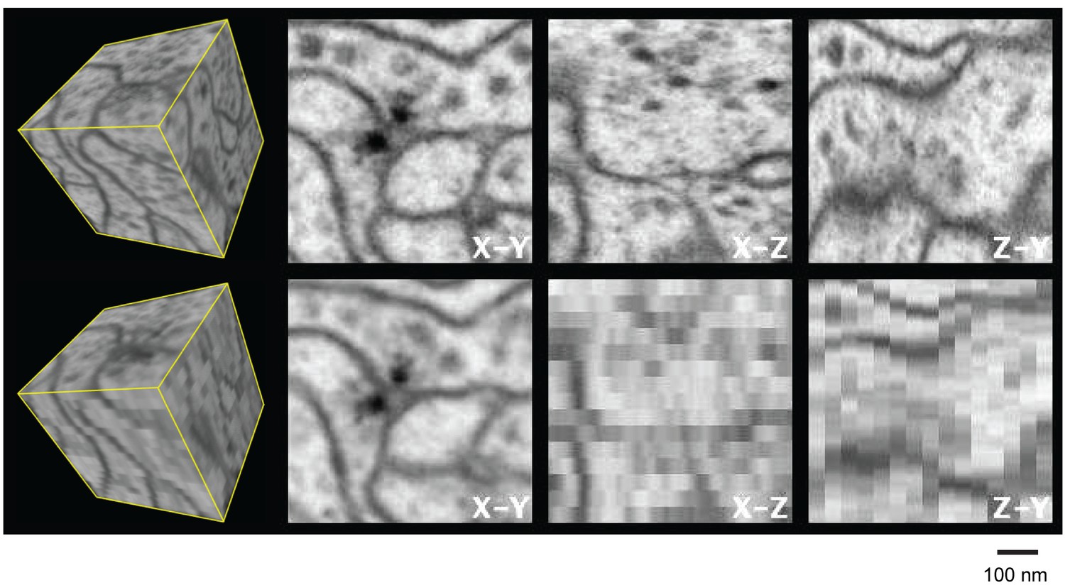
Three orthogonal views of a (600 nm)3 block of Drosophila neuropil with isotropic 4 nm voxels and anisotropic (4 x 4 x 40 nm3) voxels derived from the isotropic data to emulate 40-nm section data.
Video 1 corresponds to this Figure. Scale bar, 100 nm.
Figure 3
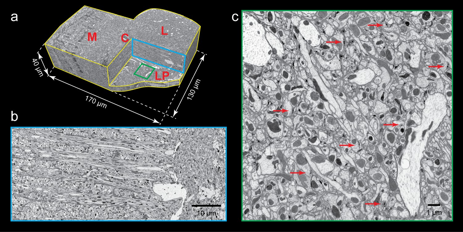
FIB-SEM images of Drosophila optic lobe.
(a) A cropped FIB-SEM volume showing medulla (M), lobula (L), lobula plate (LP), and chiasm (C). (b) An enlargement of the blue cross-section in (a) showing a re-sliced y-z plane. Scale bar, 10 µm. (c) An enlargement of the green box in (a) showing a re-sliced x-z plane where very fine neural processes are visible. Red arrows indicate synaptic structures. Scale bar, 1 µm.
Figure 4
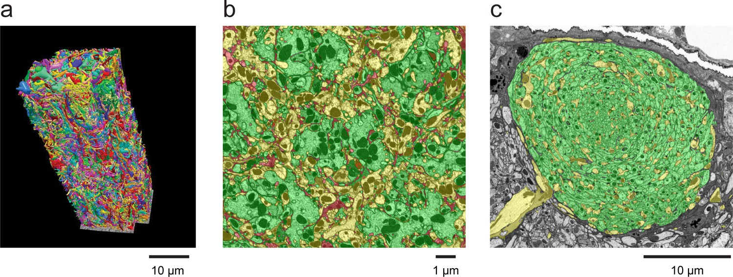
Examples of densely reconstructed data.
(a) A 3D rendering of seven columns of the medulla of the Drosophila optic lobe from FIB-SEM showing reconstructed neurons from a ~ 30,000 µm3 volume. This reconstruction, which required over five man-years of effort, was ~3–5x faster than a comparable optic lobe reconstruction using an image stack from serial-section TEM, for which we have reconstructed a single medulla column (Takemura et al., 2013). Scale bar, 10 µm. (b) A cross-section of the neuropil of the medulla in the optic lobe of Drosophila, showing the high degree of reconstruction completeness that is possible with FIB-SEM data. The hexagonal periodicity reflects the hexagonal pattern of the ommatidia of the fly’s retina. The colors illustrate how all neural processes have been assigned. Green indicates various identified columnar input neurons contained within this volume, and yellow indicates axons and arbors of various medulla neurons that branch into or out of this volume. The small remainder (shown in red) highlights the ‘left over’ parts, including unidentified and orphaned fragments of neurons and glial processes. Well over 90% of the neuropil volume could be reconstructed and assigned to specific neurons. Scale bar, 1 µm. (c) Cross-section of the neuropil of the mushroom body of Drosophila. Notice that virtually all processes in this section have been identified and colorized green (to denote Kenyon cells) or yellow (for other identified mushroom body neurons). The only ‘left over’ uncoded processes are a few thin fragments dispersed within the mushroom body boundary that could not be confidently assigned to a specific cell. The mushroom body volume was comparable to the seven-column medulla volume and required a comparable reconstruction effort. Scale bar, 10 µm. Image process, segmentation, and 3D rendering provided by the Janelia FLYEM team, see Acknowledgements.
Figure 5

Overview of ultrathick partitioning and imaging results.
(a) X-ray micro-CT of Drosophila brain cross-section shows central complex structures (the doughnut-shaped structure at center is the ellipsoid body). Yellow planes show locations of hot knife cuts at 20 µm intervals. Red highlighted area shows FIB-SEM imaged volume covering nine hot knife sections (#22-30 in our notation). Example light micrographs of Section #26 and #27 are shown (dashed box shows FIB-SEM imaged volume in each). (b) Each hot knife section is flat embedded against a PET laminate, individually mounted on a metal stud, and laser trimmed to dimensions suitable for efficient FIB-SEM imaging (Hayworth et al., 2015). (c) X-ray micro-CT of individually-mounted hot knife section showing laminar structure. All sections are micro-CT imaged as a quality control prior to FIB-SEM imaging. (d) Z-Reslice through FIB-SEM imaged volume of section #26. Blue box shows location of volume stitch test in protocerebral bridge region. Scale bar, 40 µm. (e) Result of volume stitch test in protocerebral bridge region. The FIB-SEM volumes of corresponding regions of adjacent hot knife sections #26 and #27 were computationally flattened and stitched to produce a single FIB-SEM volume suitable for tracing (Hayworth et al., 2015). Red dashed line shows stitch line. This stitched volume is available as Video 8. Scale bar, 2 µm.
Figure 6

Improved FIB-SEM resolution reveals more detailed cellular structures in biological samples.
Typical images of (a) Drosophila central complex and (b) Chlamydomonas reinhardtii, using standard 8 × 8 × 8 nm3 voxel imaging condition are shown in the top panels. The bottom panels show the corresponding high-resolution images at 4 × 4 × 4 nm3 voxel. Scale bar, 1 µm. Inset scale bar, 200 nm.
Figure 7
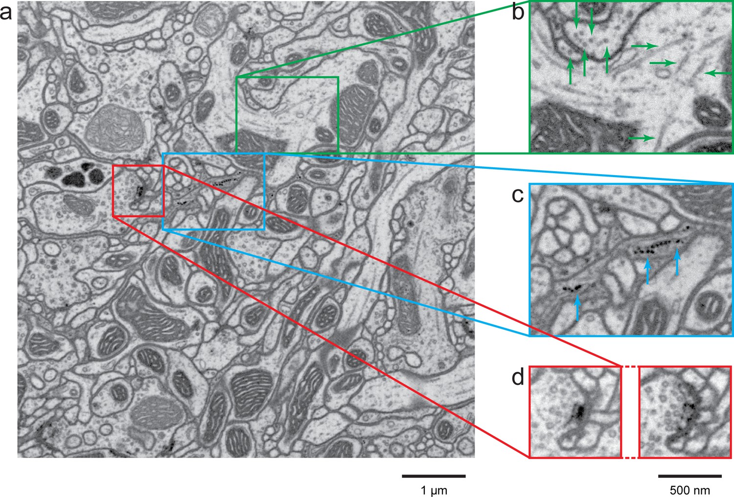
A high-resolution image (4 × 4 × 4 nm3) of a Drosophila protocerebral bridge (in the central complex) reveals fine details of various organelles.
(a) an 8 × 8 µm2 area overview; (b) end-on and side views of microtubule, indicated by green arrows; (c) polyribosomes attached to the endoplasmic reticulum, indicated by blue arrows; and (d) synaptic vesicles, presynaptic T-bar, and postsynaptic density, shown in two different z planes. Video 4 shows the corresponding full z stack. Scale bar, 1 µm in (a) and 500 nm in (b)-(d).
Figure 8

Isotropic high-resolution data offer easy visualization of 3D structures through arbitrary slices.
(a) Two orthoslices (x–y and x–z) from nucleus accumbens in a sample of adult mouse brain. (b) Specific slices of the same volume as in (a) provide easy viewing of Golgi in the context of other nearby organelles. Matching arrows in (a) and (b) indicate the same ROI’s through different slice views, (c) Polyribosomes and nuclear pores (arrow) at the nuclear envelope of a Chlamydomonas reinhardtii. The 3D rendering was generated by thresholding a maximum intensity projection where brighter yellow (polyribosomes) indicates higher intensity of backscattered electrons due to stronger staining than darker yellow (nuclear pores). Scale bar 1 µm and 100 nm.
Figure 9
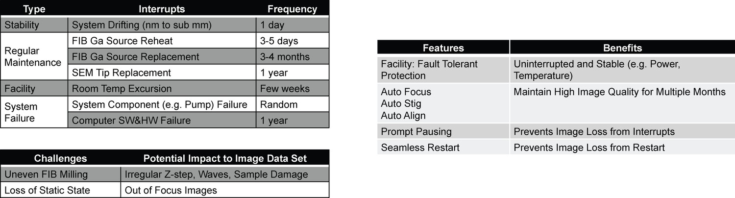
Major challenges to long-term reliability and stability of FIB-SEM systems.
(a) System failure modes with different frequencies of occurrence and resume challenges. (b) Corresponding customized solutions.
Figure 10

Cross-sectional diagram of closed-loop control set-up for FIB milling, showing the inner and annular Faraday cups.
A beam deflector provides fine-tuning to steer the positively charged FIB beam into the inner Faraday cup. Feedback currents from specimen, annular, or inner Faraday cup can be used to control the FIB beam milling position for a targeted removal rate. Inset at upper right corner shows a picture of ‘Feiss’ system in which an FEI Magnum FIB column is mounted perpendicularly to the SEM column in a Zeiss Merlin SEM.
Figure 11
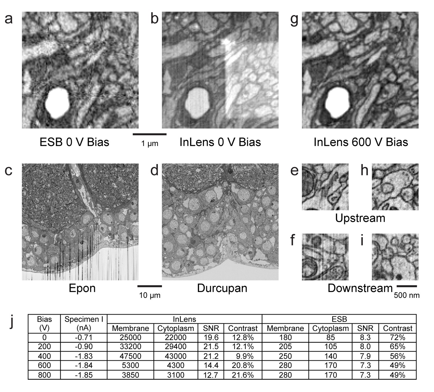
Images of ultra-thin section of Drosophila brain on silicon substrate highlight the advantages of our specimen bias scheme.
(a) EsB signals had higher contrast but lower signal-to-noise ratio (SNR) compared to InLens (b). With 600 V bias (g), InLens contrast substantially increased, with only a small drop in SNR. In addition, artifacts such as electron burn marks were eliminated by the positive bias. Streak artifacts depend on embedding resin; Epon (c) is far less satisfactory than Durcupan (d). Streak artifacts are less prominent upstream (e,h) and more prominent downstream of the ion milling (f). A 600 V bias can eliminate the surface topography contrast that makes these streaks visible (i). (j) Specimen bias effects are quantified through SNR and contrast. SNR was calculated as (Nm - Nc)/sqrt((Nm + Nc)/2), where Nm and Nc are electron counts of membrane and cytoplasm respectively. Contrast was calculated as (Nm - Nc)/((Nm + Nc)/2). Scale bar, 1 µm in (a), (b) and (g), 10 µm in (c) and (d), 500 nm in (e), (f) (h), and (i).
Figure 12 with 1 supplement
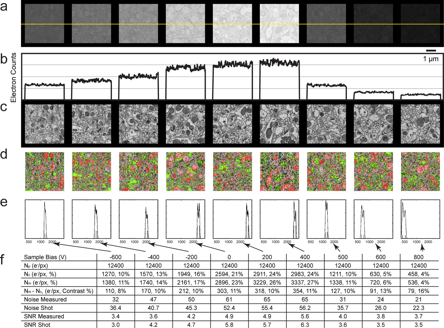
Analysis of specimen bias effects in FIB-SEM applications.
(a) Series of constant grey scale FIB-SEM images at various bias conditions from −600 to 800 V with identical electron count grey scales. Landing energy was also fixed at 1.2 keV. (b) Intensity profile of the yellow line in (a) illustrates the electron counts as a function of bias voltage over a 0 to 4000 count range. (c) Images of (a) after grey scale adjustment. (d) Red and green thresholds indicate Nm and Nc. Histogram of counts per pixel (e), Sample bias, SNR and contrast (f) of the corresponding images. Scale bar, 1 µm in (a), (c), and (d).
Figure 12—figure supplement 1

Enlarged figures from Figure 12 to illustrate the manual thresholding method of Nm and Nc estimates.
(a) Inverted grey scale FIB-SEM image as in Figure 12c. (b) Red and green thresholds were manually adjusted so that ~50% of cell membranes were colored in red and ~50% cell cytoplasm (excluding mitochondria) was green as in Figure 12d. (c) Intensity profile of the yellow line in (a). Red threshold of 720 indicates the average cell membrane electron count where the green threshold of 630 indicates the average cell cytoplasm electron count. (d) Histogram of counts per pixel, red and green vertical lines indicate cell membrane and cytoplasm electron mounts as in Figure 12e. Scale bar, 1 µm in (a) and (b).
Figure 13
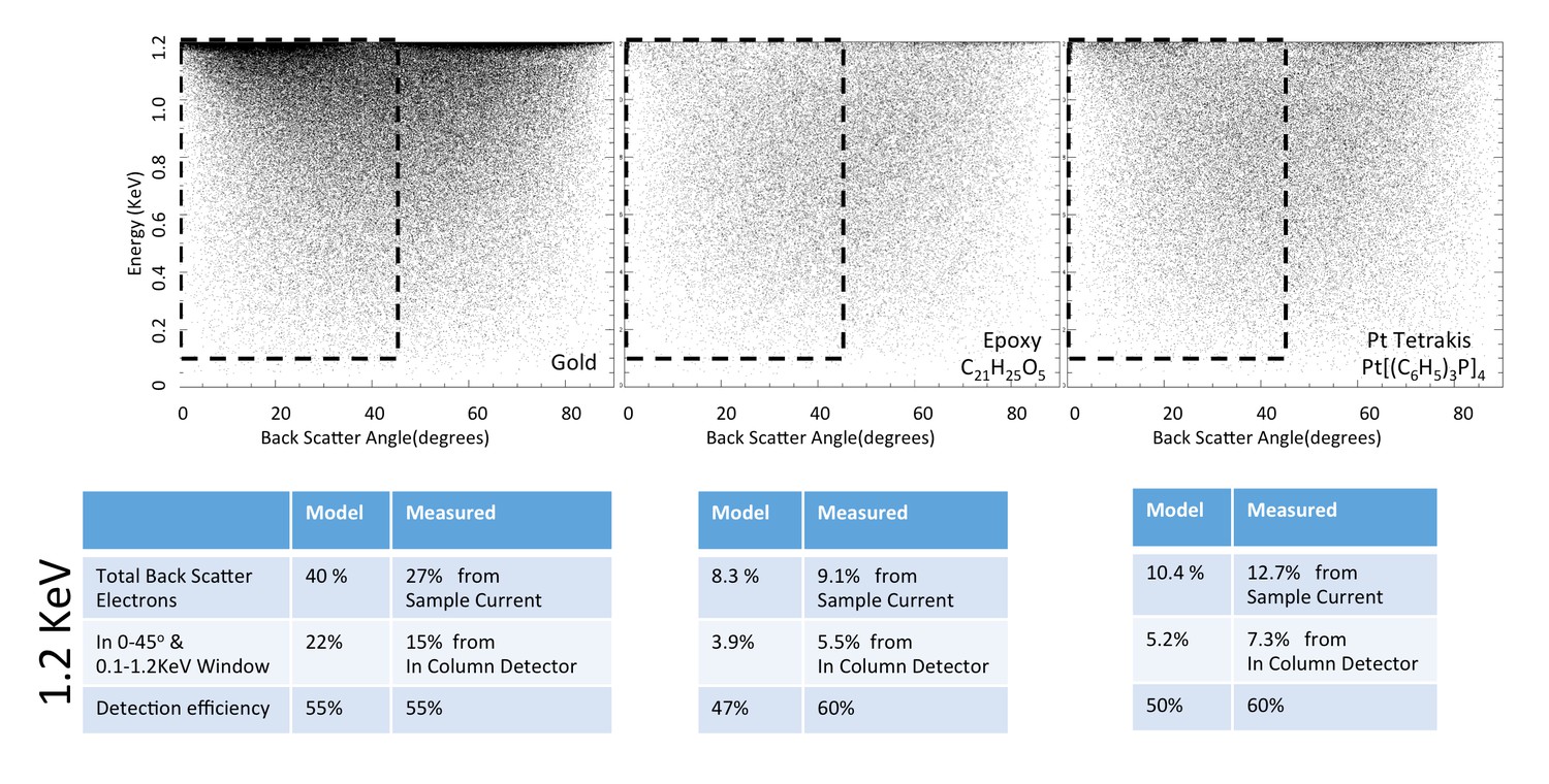
Energy and angle distribution of backscattered electrons for 1.2 keV primary electrons impinging on a reference gold, epoxy and Pt Tetrakis sample with 15% by weight of high Z element.
The measured and modeled values are in rough agreement (within 30%). Both suggest that about 50% of the backscattered electrons are detected.
Figure 14
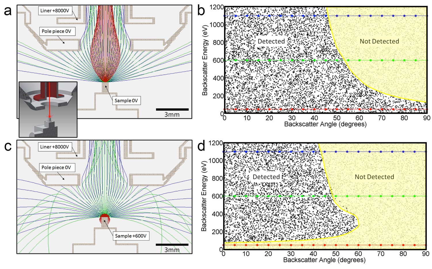
Positive bias applied to the sample suppresses secondary electrons but leaves most backscattered electrons unaffected.
In effect, this converts the SEM’s InLens ‘secondary’ detector into an efficient high-bandwidth backscatter detector well suited for FIB-SEM. (a) Electron flight simulation (using SIMION software package) showing paths of 1.1 keV (blue), 600 eV (green), and 50 eV (red) electrons emerging from an unbiased sample surface at a range of angles (−90o to 90o in 5o increments). After emerging from the sample surface, electrons are attracted by the +8 kV liner tube of the Zeiss Gemini column. (Kumagai and Sekiguchi, 2009) Inset shows the 3D CAD model that this simulation was based on. (Only electrostatic elements were modeled, not the magnetic field of the objective lens.) The lowest energy electrons (red) are all funneled up the column and thus potentially impact the InLens detector of the Gemini column. Here, we assume that all electrons that make it into the liner tube are in fact detected. For higher energy electrons (blue and green) only the central angles (−45° to 45°) are detected. (b) 10,000 electrons paths were simulated in the same model, covering a uniform range of starting energies (0 to 1.2 keV) and angles (−90° to 90°), allowing the detected vs. non-detected regions in energy vs. angle space to be plotted. All electrons below 100 eV are detected (i.e. make it into the liner tube) in this 0 V bias condition. 1.1 keV (blue), 600 eV (green), and 50 eV (red) electrons simulated in (a) are superimposed on this plot for cross-reference. (c) Same simulation as in (a) but with +600 V bias on the sample. This has a dramatic effect on the paths of the lowest energy (red) electrons, which are all pulled back onto the sample. (d) This filtering of low-energy (secondary) electrons is clearly seen in this corresponding energy vs. angle detection plot. Comparing (d) to (b) one can see that sample bias has only slight effect on the detection of higher energy electrons. The overall detection efficiency is determined by this acceptance mask, combined with the backscattered electrons distribution of Figure 13.
Figure 15
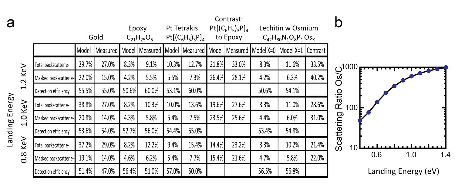
Comparison of Monte Carlo model and measurements: effects of primary landing energy on total and detected-fraction backscattered electrons.
(a) Table of results of Monte Carlo model and measurements of backscattered electrons at different landing energies, for the three reference samples and a model for an osmium-stained lipid. At lower landing energies, the contrast between stained and unstained sample drops rapidly, consistent with the increased carbon cross-section vs that of osmium at low energies. Curve is from NIST elastic scattering data. (b). With typical sample stoichiometry of 100 carbon atoms per high Z stain atom, the signal vanishes rapidly below 600 eV.
Figure 16
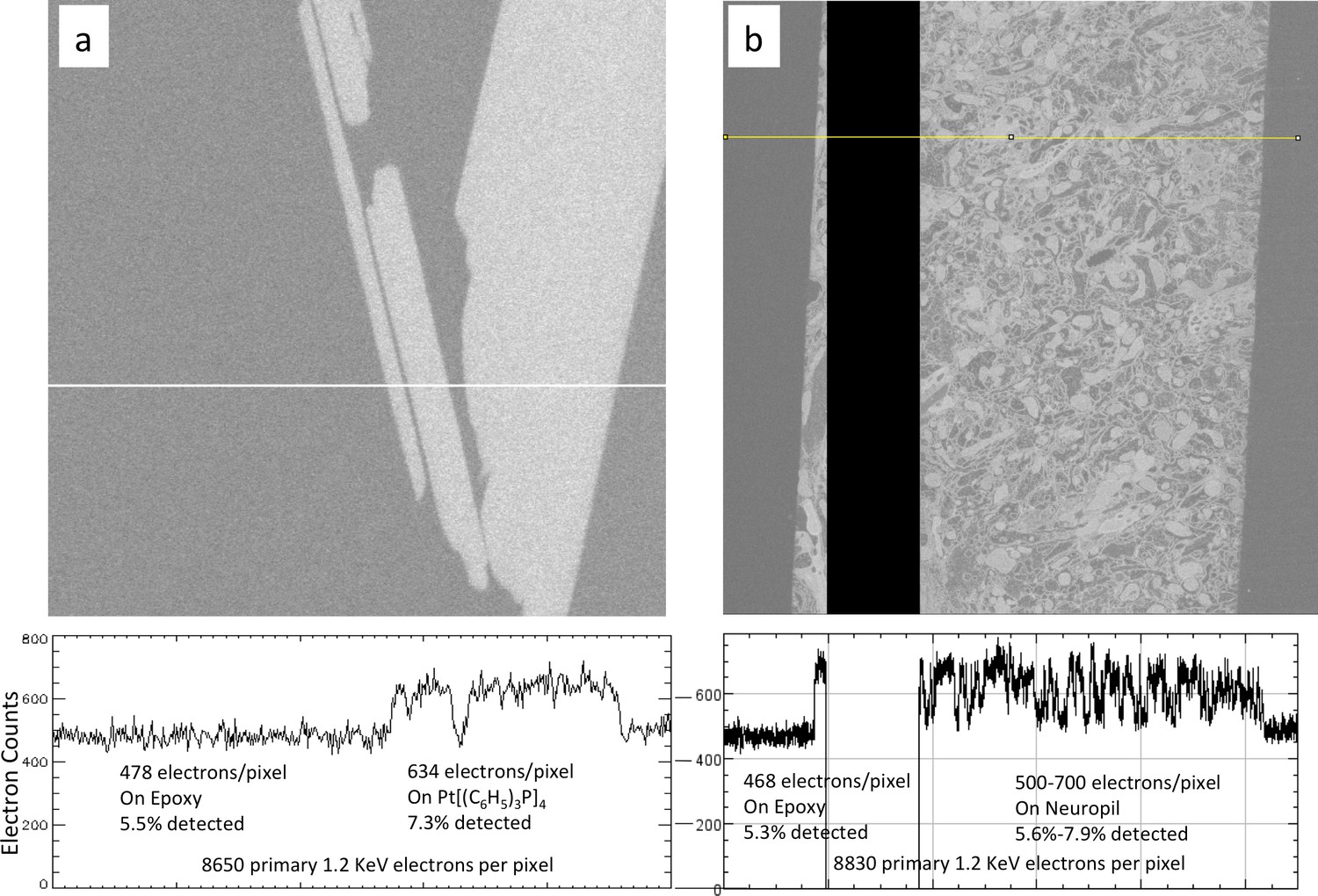
Calibration of sample osmium concentration using reference Pt Tetrakis standard.
(a) Signal from epoxy and an embedded Pt Tetrakis sample which yield about 5.5% and 7.3% detected backscatter electrons, respectively, from the 8650 incoming electrons on each pixel. The average differential of ~150 electrons is subject to shot noise of about 22 electrons, giving an SNR of 8. One can see in (b) that typical fly neuropil prepared using the PLT procedure with a non-quantified osmium stain concentration has about the same contrast and SNR and can be calibrated against this Pt Tetrakis standard.
Figure 17

Effect of landing energy on the point spread function based on Monte Carlo simulations.
(a,b,c).Monte Carlo simulation of backscattered electrons at different landing energies. Lower landing energy generates smaller sampling volume (implying better resolution), but with reduced contrast and SNR, as discussed in (d,e). A better measure of resolution is to model a step edge in staining from xOs = 0 to xOs = 1. The step can be lateral and shows a small transition region of less than 1 nm for about half of the signal. The sensitivity to a depth transition in staining is more gradual, with a P50 value of 5 nm for 800 eV landing energy and 11 nm for 1.2 keV landing energy. Note that the simulations assume a primary beam with zero lateral spread. The actual resolution is convolved by the actual beam width.
Figure 18
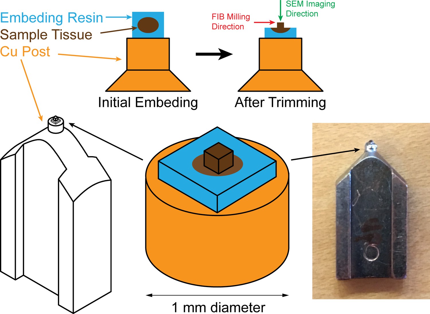
Sample mounting and trimming diagrams for FIB-SEM: sample (colored in brown) embedded in resin (colored in blue) is mounted onto a Cu stud (colored in orange), embedding resin is then trimmed off to expose the sample.
The green arrow pointing down indicates the scanning SEM beam which is perpendicular to the FIB milling direction indicated by the red arrow.
Figure 19
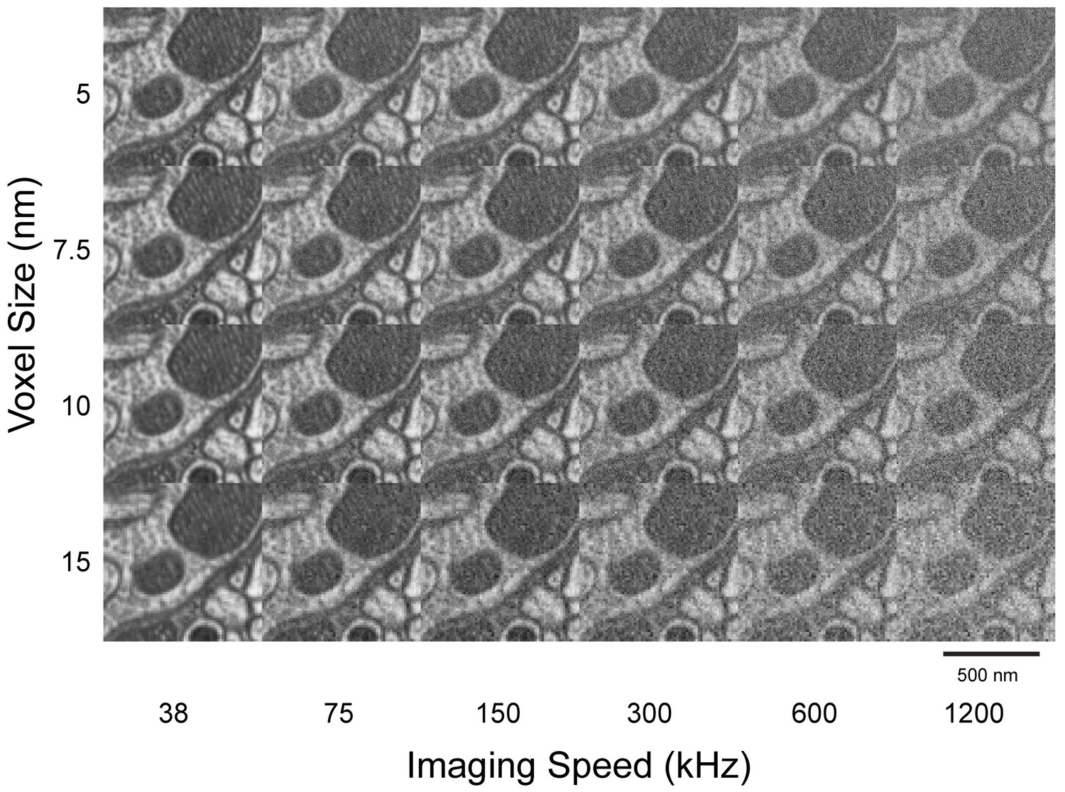
Imaging speed and voxel size study to determine optimal condition for neuronal circuit reconstruction.
A high-resolution (5 nm) image stack was first acquired at low imaging speed (38 kHz). Corresponding larger voxel and more rapidly acquired images were emulated by binning and adding shot noise through software. A condition of around 8 nm and 300 kHz was found to optimize traceability and throughput. Scale bar, 500 nm.
Videos
Video 1
Three-dimensional x,y,z data showing 4 nm voxels over 600 nm range of Drosophila neuropil with isotropic resolution (top row), and a section where the data is binned together in z to form 4 x 4 x 40 nm3 voxels, to emulate standard TEM sections.
https://doi.org/10.7554/eLife.25916.003
Video 2
Re-sliced view of Drosophila optic lobe showing medulla (left), lobula (upper right), lobular plate (lower right). 150 × 64 × 40 µm3 region with 10x zoom, 8 × 8 × 8 nm3 voxel.
https://doi.org/10.7554/eLife.25916.007
Video 3
Re-sliced views of a hot knife slab containing the Drosophila central complex at various zoom levels.
The left panel shows the entire slab at 512 × 512 × 64 nm3 voxel. The center panel shows a cropped region at the bottom of fan shape body (FB) with 64 × 64 × 64 nm3 voxel. The right panel shows a cropped region in FB with 16 × 16 × 16 nm3 voxel.
Video 4
Detail of synapse in Drosophila protocerebral bridge showing multiple post synaptic contacts.
https://doi.org/10.7554/eLife.25916.013
Video 5
Nucleus accumbens of a mouse brain.
https://doi.org/10.7554/eLife.25916.015
Video 6
Whole Chlamydomonas reinhardtii.
https://doi.org/10.7554/eLife.25916.016
Video 7
Flagella structure of a Chlamydomonas reinhardtii.
https://doi.org/10.7554/eLife.25916.017
Video 8
Result of volume stitch test in Drosophila protocerebral bridge region between hot knife sections #26 and #27.
https://doi.org/10.7554/eLife.25916.018Additional files
-
Source code 1
3D FIB-SEM LabVIEW codes.
- https://doi.org/10.7554/eLife.25916.031
Download links
A two-part list of links to download the article, or parts of the article, in various formats.
Downloads (link to download the article as PDF)
Open citations (links to open the citations from this article in various online reference manager services)
Cite this article (links to download the citations from this article in formats compatible with various reference manager tools)
Enhanced FIB-SEM systems for large-volume 3D imaging
eLife 6:e25916.
https://doi.org/10.7554/eLife.25916


