Olfactory receptor neurons use gain control and complementary kinetics to encode intermittent odorant stimuli
- Yale University, United States
Figures
Figure 1 with 4 supplements
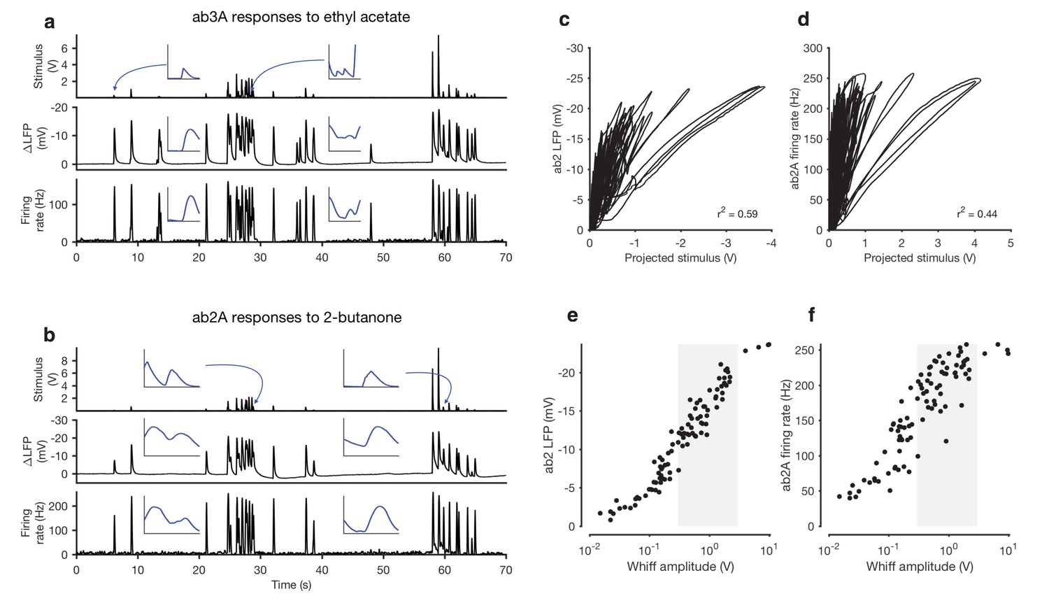
Adaptation and saturation modulate ORN responses to broadly distributed naturalistic stimuli.
(a) Ethyl acetate odorant (top) elicits LFP (middle) and firing rate (bottom) responses from a ab3A ORN. (b) 2-butanone odorant (top) elicits LFP (middle) and firing rate (bottom) responses from a ab2A ORN. Insets in (a–b) show pairs of whiffs and the LFP and firing rate responses they elicit on an expanded timescale. All pairs of insets are shown at the same scale, for 400 ms around a whiff. (c) ab2 LFP responses vs. projected stimulus. (d) ab2A firing rate vs. projected stimulus. (c) and (d) show that ORN responses differ significantly from linearity. (e) ab2 LFP responses vs. whiff amplitude. (f) ab2A firing rate vs. whiff amplitude. n = 15 trials from 2 ORNs. 101 whiffs shown in (e–f).
Figure 1—figure supplement 1
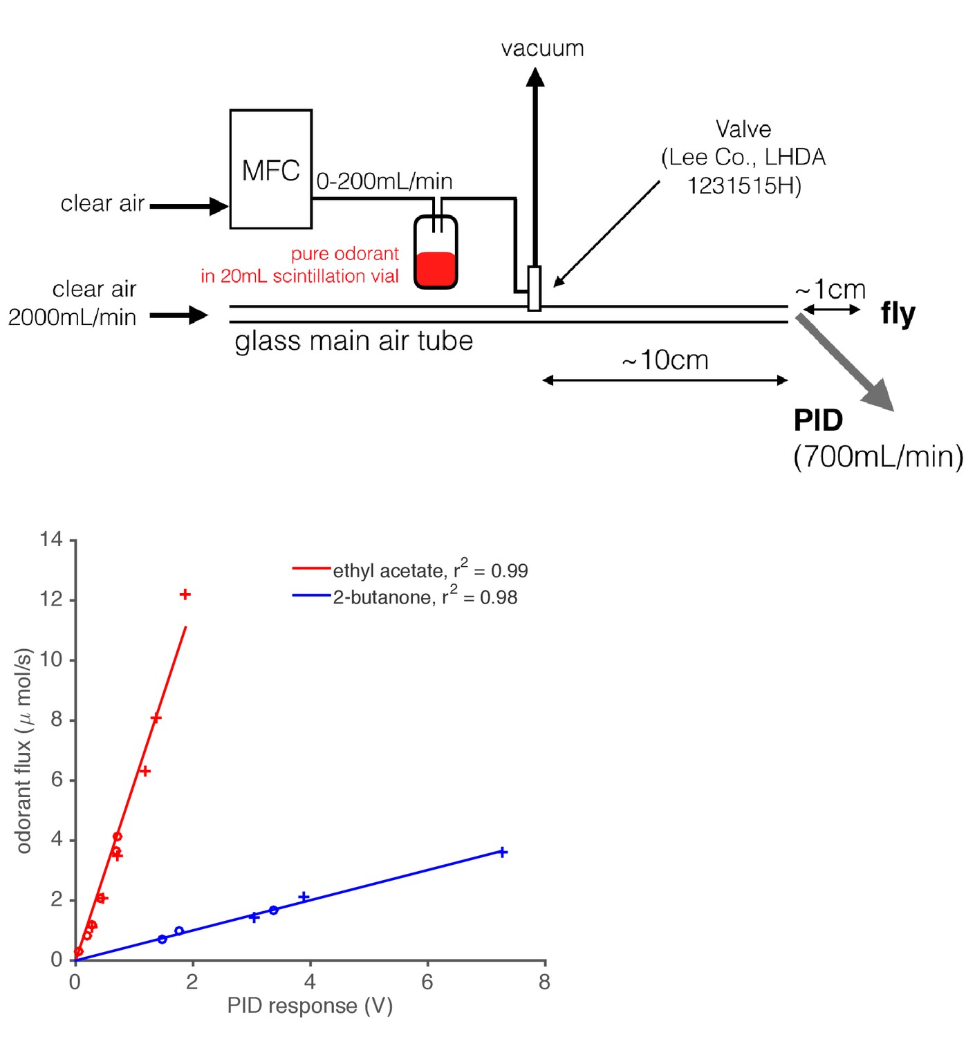
Diagram of odor delivery device and calibration of Photo-Ionization Detector (PID).
1 mL of pure odorant was placed in a 20 mL scintillation vial with a screw top. A computer-controlled Mass Flow Controller (MFC) forced air through this vial, which created an odorized airstream. This airstream was either directed into the main air flow or to waste (vacuum) using a solenoid valve. A PID (inlet needle at the outlet of the main air tube) recorded the gas phase concentration of the odorant stimulus as it was presented to the fly. We calibrated the PID by depleting a fixed, known volume of pure odorant at various flow rates, and integrating the resultant PID signal. Using the known densities and molar masses of these monomolecular odorants, we built maps from PID response in Volts onto the absolute odorant flux. This relationship was found to be linear for the two odorants tested.
Figure 1—figure supplement 2
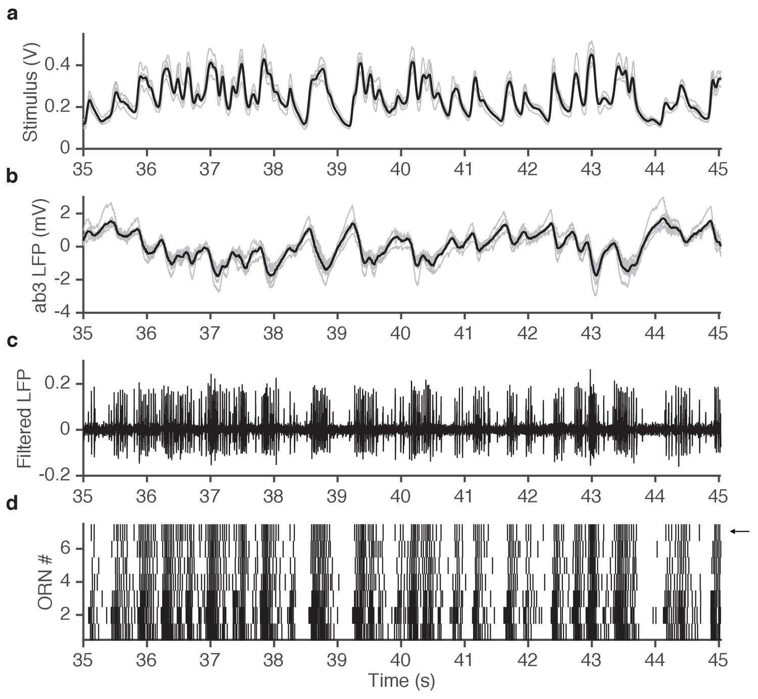
Example of simultaneously acquired primary data (ab3A responses to ethyl acetate stimulus).
(a) Seven repetitions of fluctuating ethyl acetate stimulus (each gray trace is from a presentation to a different ab3A neuron in a different sensillum; mean shown in black). (b) Raw voltage recording from 7 different ab3 sensilla. (gray traces, one from each neuron; mean shown in black). (c) One of the traces in (b) is filtered to visualize spikes. Note that spikes from the ab3A neuron are typically larger than spikes from the ab3B neuron, enabling us to sort them and measure the response of a single neuron in vivo. (d) Raster of ab3A spikes for 7 different ORNs. Arrow indicates trace shown in (c).
Figure 1—figure supplement 3
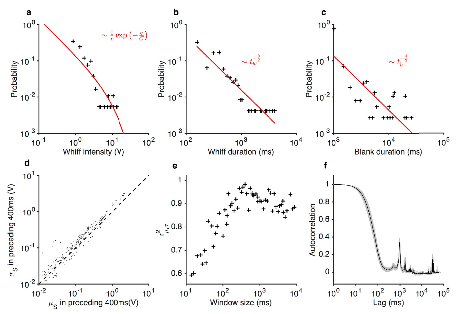
Statistics of the ethyl acetate stimulus with naturalistic temporal structure.
(a) Distribution of whiff intensities. (b) Distribution of whiff durations. (c) Distribution of blank durations. Predicted distributions from Celani et al. (2014) are shown in red lines (a–c). is the odor concentration (whiff intensity). and are whiff and blank durations. (d) Mean vs. standard deviation of stimulus, computed in 400 ms non-overlapping blocks. (e) Correlation between mean and standard deviation of stimulus as a function of window length. Peak correlation observed for timescales ~400 ms. (f) Autocorrelation function of the stimulus. Shading indicates standard deviation across trials.
Figure 1—figure supplement 4
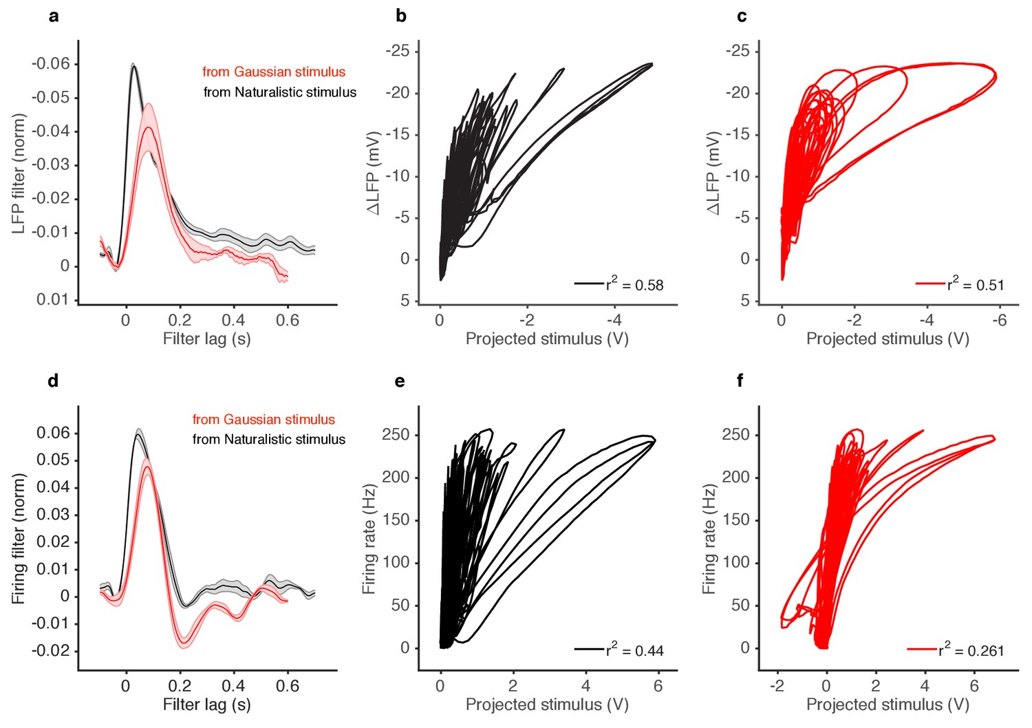
Deviations from linearity persist even when filters extracted from Gaussian stimuli are used to project naturalistic stimulus.
(a) LFP filters for ab2A ORNs responding to 2-butanone, extracted either form naturalistic stimuli (black) or from Gaussian stimuli (red). (b) LFP responses to naturalistic stimulus vs. stimulus projected through filter computed from naturalistic stimulus (Black filter in a). (c) LFP responses to naturalistic stimulus vs. stimulus projected through filter computed from Gaussian stimulus (red filter in a). (d) Firing rate filters for ab2A ORNs responding to 2-butanone, extracted either from naturalistic stimuli (black) or from Gaussian stimuli (red). (e) Firing rate responses vs. stimulus projected through filter computed from naturalistic stimulus (black filter in d). (f) Firing rate responses vs. stimulus projected through filter computed from Gaussian stimulus (red filter in d).
Figure 2 with 1 supplement

Adaptation and saturation modulate ORN responses to broadly distributed naturalistic stimuli.
(a). Ethyl acetate whiffs of similar size (top) elicit ab3 LFP responses (middle) and ab3A firing rate responses (bottom) with different amplitudes. (b) 2-butanone whiffs of similar size (top) elicit ab2 LFP responses (middle) and ab2A firing rate responses (bottom) with different amplitudes. Bar graphs in (a) and (b) show that ordering in LFP and firing rate response does not correlate with whiff amplitude, but correlates with the intensity of the preceding whiff. Colors on bar graph correspond to colors in time series on the left. Deviations in LFP (c) and firing rate responses (d) from the median response vs. mean stimulus in the preceding 300 ms. Deviations in LFP (c, inset) and firing rate responses (d, inset) from the median response vs. whiff amplitude. (e) Deviations from the median of LFP responses (positive deviations: red, negative deviations: blue) as a function of the amplitude of the previous whiff and the time since previous whiff. Positive and negative deviations are significantly different (, 2-dimensional K-S test). (f) Deviations from the median of firing rate responses (positive deviations: red, negative deviations: blue) as a function of the amplitude of the previous whiff and the time since previous whiff. Positive and negative deviations are significantly different, (, 2-dimensional K-S test on firing rate deviations).
Figure 2—figure supplement 1
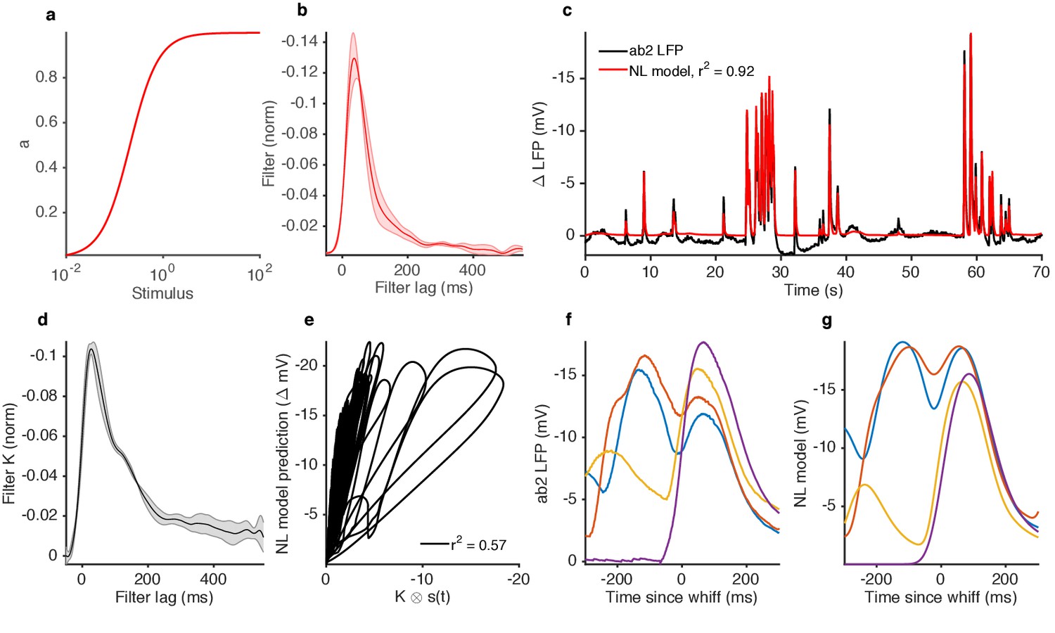
An NL model (static input nonlinearity followed by a linear filter) cannot reproduce context-dependence of LFP responses to similar-sized whiffs.
Input nonlinearity (a) and filter (b) fit to ab2 LFP responses to 2-butanone naturalistic stimulus. The input nonlinearity is a Hill function where S represents the input, and KD the half maximum value). The nonparametric filter and parametric nonlinearity are fit simultaneously in an iterative manner (see Materials and methods). (c) Comparison of ab2 LFP responses and NL model predictions. (d) Linear filter extracted from the stimulus and the NL model prediction. Note that the filter is not the same as in (b); a filter extracted from an NL model is not guaranteed to be an unbiased estimate of the true one. (e) NL model responses vs. naturalistic stimulus projected through filter in (d), showing that the NL model shows deviations from linearity similar to what is observed in the data (cf. Figure 1c). (f–g) Context dependence of response in the ab2 data and model. (f) ab2 LFP responses to whiffs of similar size (same data as in Figure 1h). Note that the responses to isolated whiffs (purple, yellow) are larger than the responses to repeated whiffs (red, blue). (g) NL model responses to these whiffs. Note that the responses to isolated whiffs (purple, yellow) are smaller than the responses to repeated whiffs (red, blue), the opposite of the trend visible in the data.
Figure 3 with 3 supplements
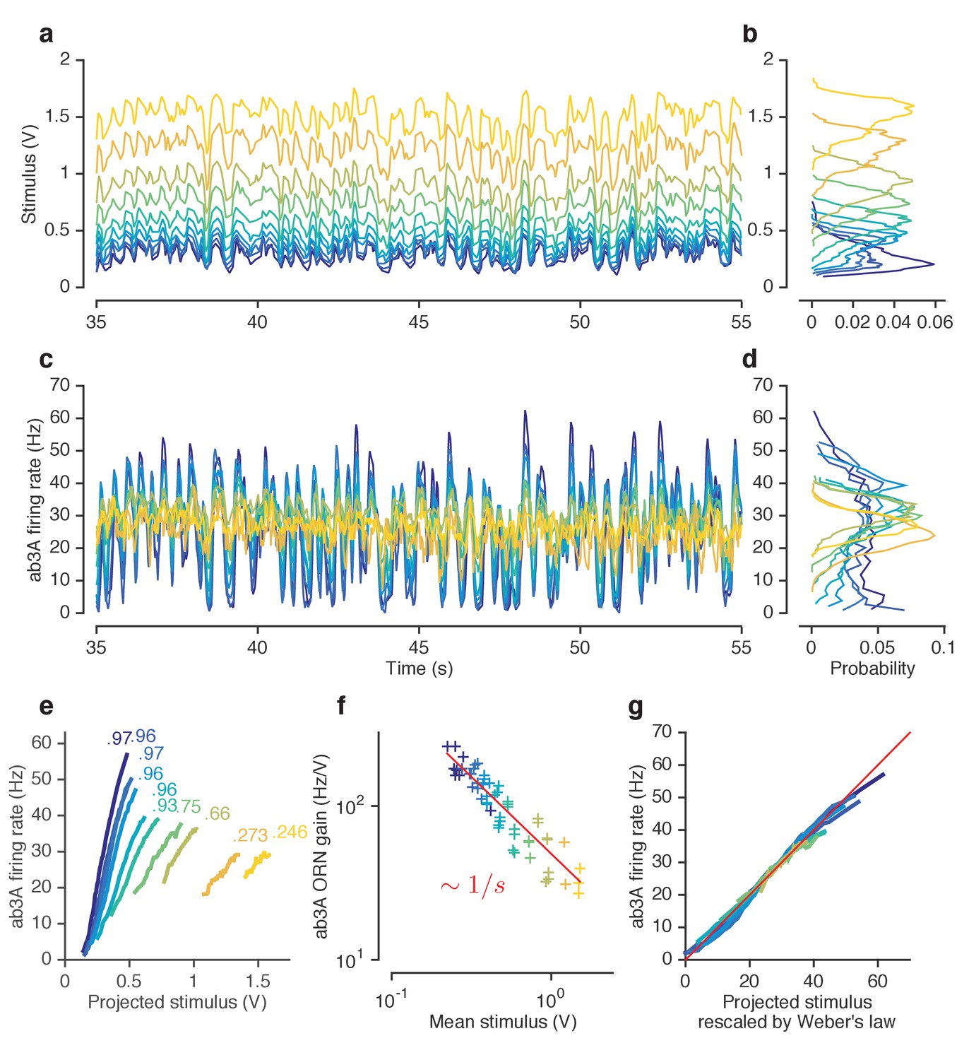
ORNs decrease gain with stimulus mean, consistent with the Weber-Fechner Law.
(a) Ethyl acetate stimuli with different mean intensities but similar variances. Stimulus intensity measured using a Photo-Ionization Detector (PID), units in Volts (V). Colors indicate mean stimulus intensity. (b) Corresponding stimulus distributions. (c) ab3A firing rate responses to these stimuli. (d) Corresponding response distributions. (e) ORN responses vs. stimulus projected through linear filters. Colored numbers indicate between linear projections and ORN response. (f) ORN gain vs. mean stimulus for each trial. Red line is the Weber-Fechner prediction () (g) After rescaling the projected stimulus by the gain predicted by the red curve in (f), and correcting for an offset, ORN responses collapse onto one line. n = 55 trials from 7 ORNs in 3 flies. All plots except (f) show means across all trials. (f) shows individual trials.
Figure 3—figure supplement 1
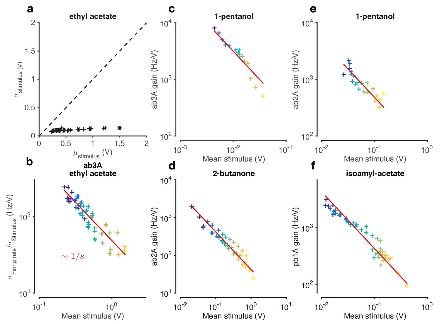
Weber-Fechner Law broadly observed across odor-receptor combinations.
(a) Standard deviation vs. mean of ethyl acetate stimulus in Figure 1. (b) ORN gain estimated by the ratio of standard deviation of firing rate to standard deviation of stimulus, vs. mean stimulus in each trial. This model-free estimate of ORN gain ignores kinetics of response, but returns similar estimates of the gain (cf. Figure 3f). Note that the units of gain estimated this way are the same. (c–f) ORN gain as a function of mean stimulus for various odor-receptor combinations. In all plots, the red line is a power law with slope −1 (the Weber-Fechner Law). Data in panel a and b is the same as in Figure 3. n = 121 trials from 16 ORNs in 6 flies.
Figure 3—figure supplement 2

Ability of NL models to reproduce observed change in input-output curves.
(a–c) Static NL model responses. (a) The input nonlinearity of NL model is chosen to be a Hill function with n = 1. (b) Filter of NL model, measured directly from the data. (c) NL model responses vs. projected stimulus. While these curves appear to change slope with increasing mean stimulus, mean responses also tend to increase (purple … yellow). (d–f) Varying NL model responses, where the KD of the input nonlinearity is allowed to vary with the mean stimulus. (d) Input nonlinearities for stimuli with different mean (colors). The KD of each curve is set to the mean stimulus of that trial. (e) Filter of NL model, same as in (b). (f) Model responses vs. projected stimulus. Note that, like in the data (cf. Figure 2e), the mean response remains relatively invariant with mean stimulus, and that curves get shallower with increasing mean stimulus. (g) Comparison of steady state gain (slope of functions shown in (a) and (d)) when KD is fixed (black) and when KD is allowed to vary with the mean stimulus (red). When KD is fixed, the the relationship between gain and mean stimulus approaches a power law with exponent 2 (gain ~ ). However, when varies with the mean stimulus, the steady state gain ~ , which is the Weber-Fechner Law.
Figure 3—figure supplement 3
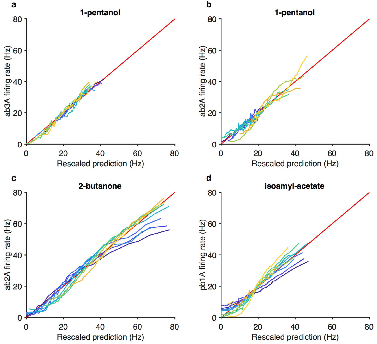
Projected stimulus rescaled by Weber-Fechner relation correlate with firing rates.
(a–d) Firing rate vs. projected stimulus rescaled by Weber-Fechner relation (as in Figure 3g) for four additional odorant-receptor combinations. Red line is the line of unity. Same data asin Figure 3—figure supplement 1c–f.
Figure 4 with 1 supplement
ORNs decrease gain with stimulus variance.
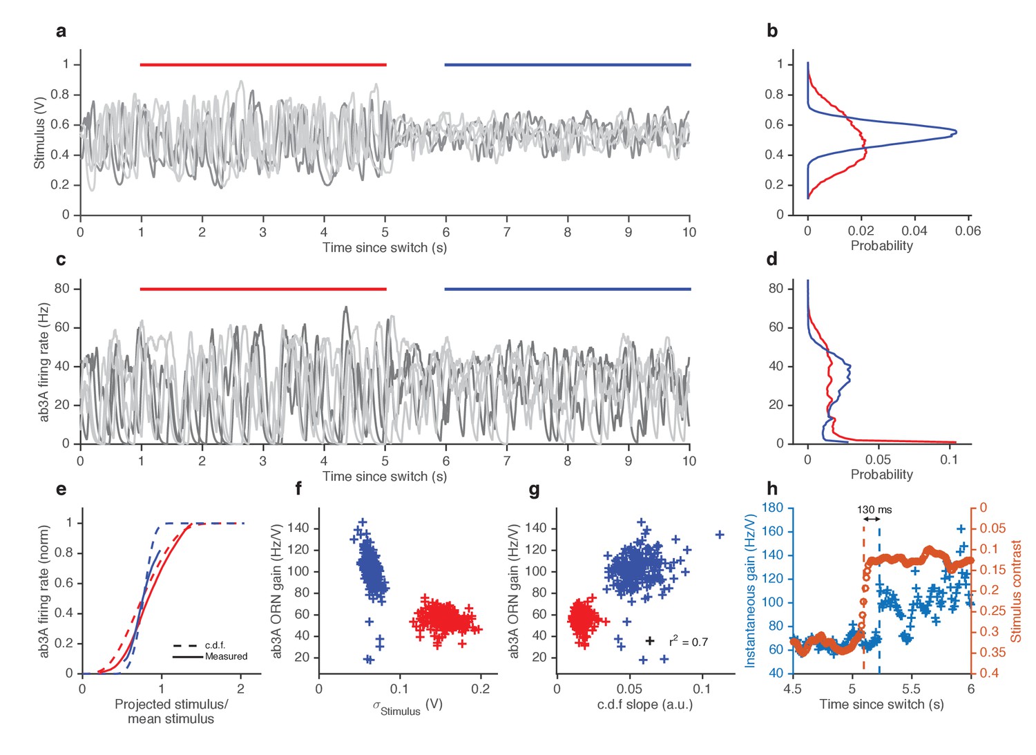
(a). Stimulus intensity of a fluctuating ethyl acetate stimulus with nearly constant mean but a variance that switches between high and low every 5 s. Five independent trials (out of 248) are plotted. (b) Distributions of stimulus intensity for the epochs of low (blue) and high (red) variance. (c) ab3A firing rate responses corresponding to the trials shown in (a) following the switch from low to high variance, which takes place at t = 0 s and from high to low, which takes place at t = 5 s. (d) Probability distributions of the response. (e) Solid lines are ORN input-output curves computed from a single filter from both low (blue) and high (red) variance epochs. Dashed lines are the cumulative distribution functions (c.d.fs) of the projected stimulus. (f) ORN gain as a function of the standard deviation of the stimulus, measured per trial for each epoch. (g) Measured gain plotted against the slope of the cumulative distribution function for each trial. (h) Instantaneous gain (blue) and stimulus contrast (orange) as a function of time since switch. Dashed lines indicate crossover times of stimulus contrast and instantaneous gain. The delay is ~130 ms. n = 248 trials from 5 ab3A ORNs in 2 flies.
Figure 4—figure supplement 1
Variance gain control in Gaussian stimuli.
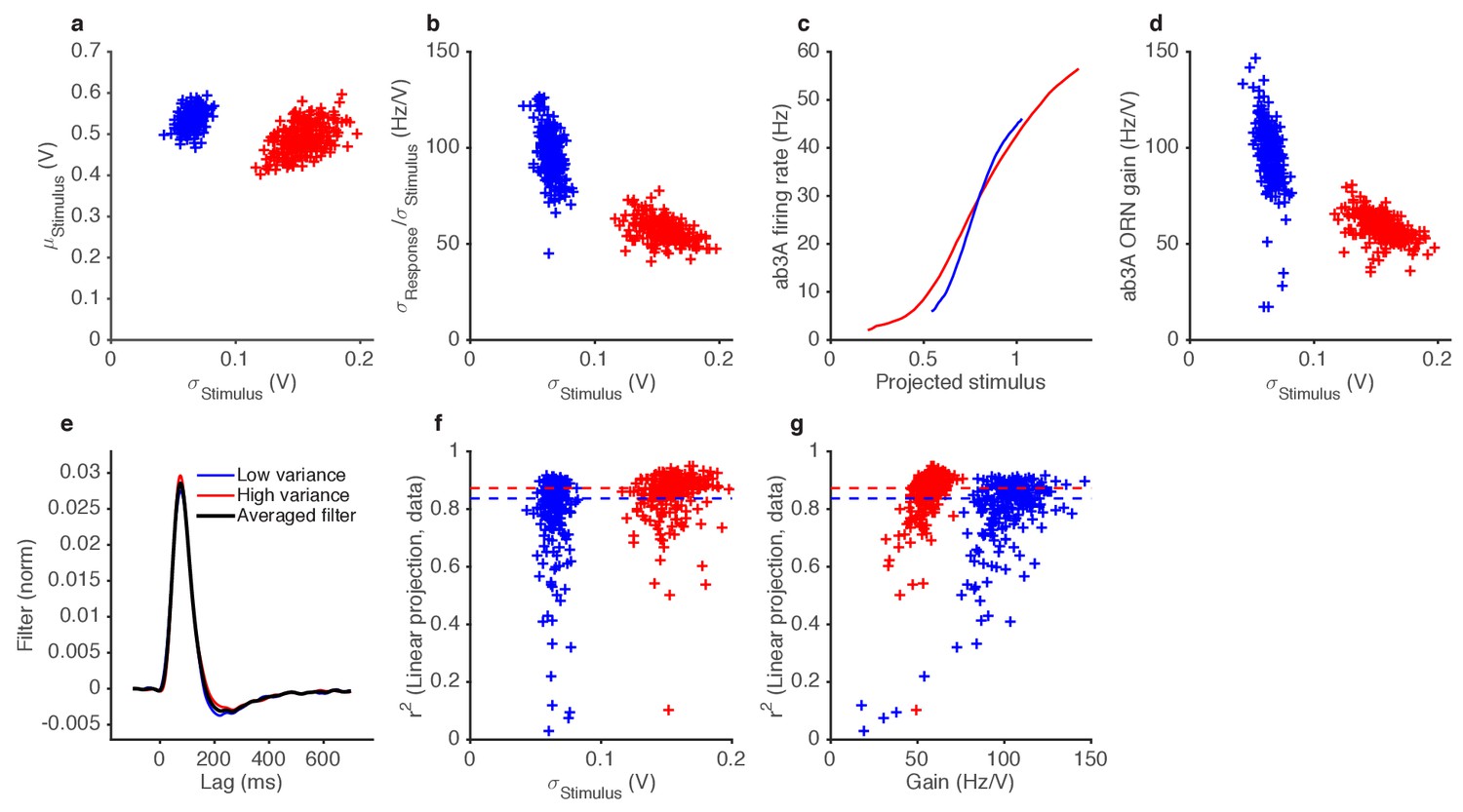
(a) While the dominant change between the two epochs is the change in variance (by construction), the low variance trials also tend to have slightly higher means. (b) ORN gain estimated by dividing the standard deviation of the response by the standard deviation of the stimulus, for each trial, vs. the standard deviation of the stimulus (cf. Figure 4f). (c) Input-output curves for the ab3A ORN uncorrected for the change in the mean stimulus. The blue curve intersects the red curve, and is steeper than the red curve, suggesting that gain during the low variance epoch is higher than the gain during the low variance epoch. (d) ORN gain during high and low variance epochs, without correcting for the change in the mean stimulus. Each trial appears in the plot as one blue point (for the low variance epoch) and one red point (for the high variance epoch). (e) Filters used in this analysis. Filters backed out of low variance (blue) or high variance (red) epochs alone are very similar. Therefore, we averaged all filters (black) and used that averaged filter to project all the stimulus in this dataset. (f) Coefficient of determination () vs. the standard deviation of the stimulus.~80% of trials had >0.8. (g) Coefficient of determination () vs. trial-wise ORN gain in the high and low variance epoch. Dashed lines in (f–g) indicate the median during the high and low variance epoch.
Figure 5 with 1 supplement
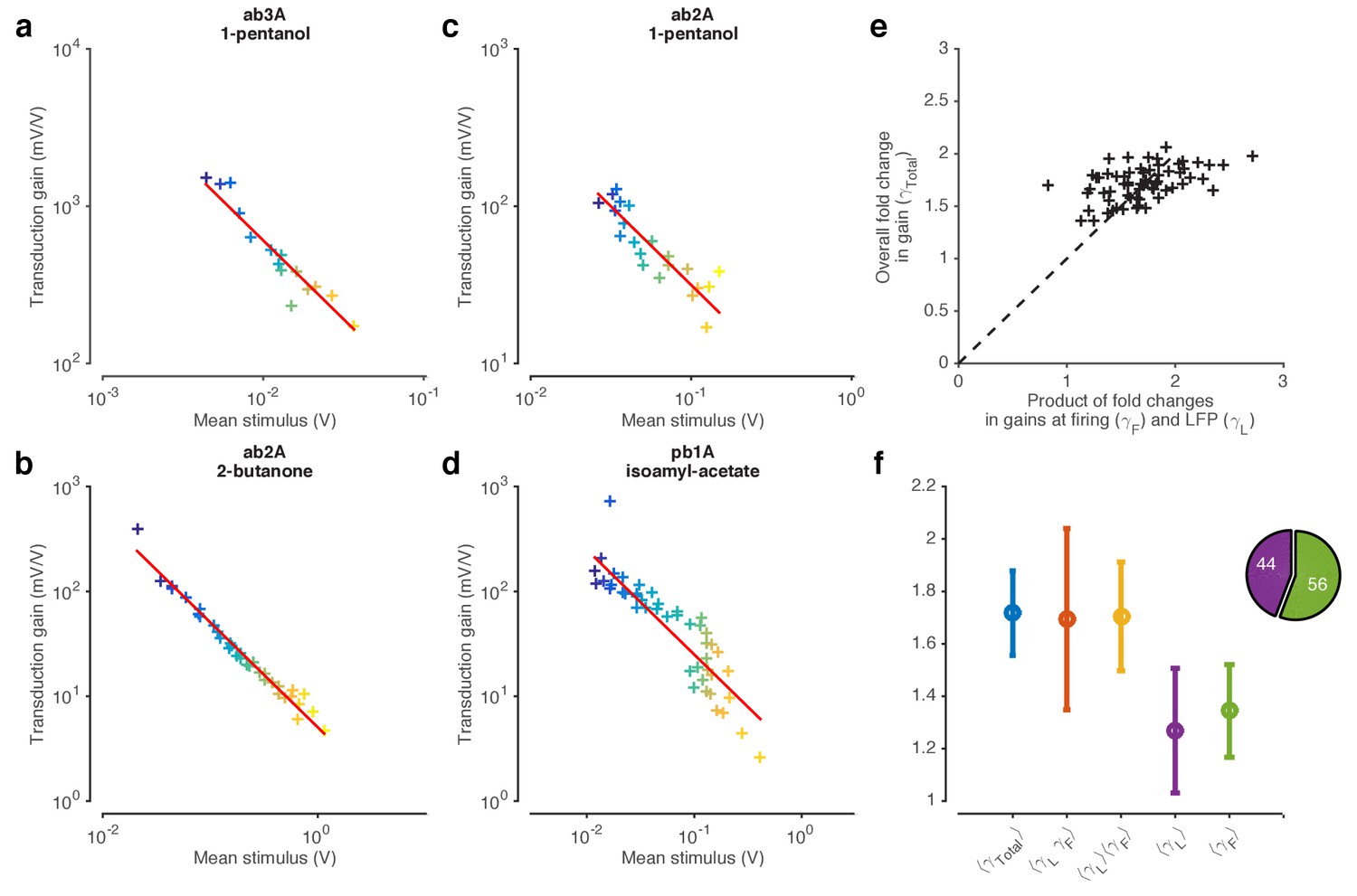
Mean gain control occurs primarily at transduction, and variance gain control occurs both at transduction and at the firing machinery.
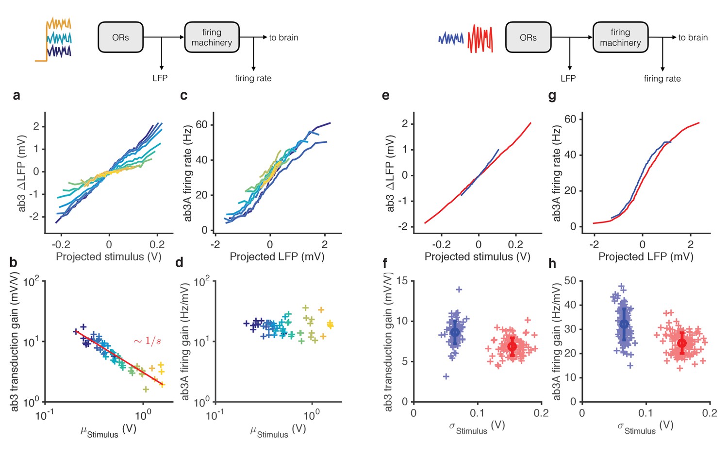
(a) Transduction input-output curves from stimulus to LFP. Colors indicate increasing mean stimulus. Filters and projections are computed trial by trial. (b) Transduction gain, measured from the slopes of these input-output curves, decreases with the mean stimulus. The red line is a power law with exponent −1, (Weber’s Law). (c) Input-output curves for the firing machine module. (d) Firing gain does not change significantly with mean stimulus. (e) Transduction input-output curves for low (blue) and high (red) variance stimuli. (f) Transduction gains in the low variance epoch are significantly higher than transduction gains in the high variance epoch (p<0.001, Wilcoxon signed rank test) (g) Input-output curves of firing machinery during low variance stimuli. (g) Firing gain during low variance epochs are significantly higher than firing gains during high variance epochs (p<0.001, Wilcoxon signed rank test). Projections of stimulus are divided by the mean stimulus in each trial to remove the small effect Weber-Fechner gain scaling. Data in this figure is same as in Figures 3 and 4. (a,c,e,g) Mean across all trials. (b,d,f,h) Individual trials.
Figure 5—figure supplement 1
LFP responses to fluctuating Gaussian ethyl acetate signals with increasing mean.
Colors correspond to increasing mean odorant stimuli (purple…yellow). The data in this figure corresponds to the data shown in Figure 3. Increasing stimulus mean decreases the variance of the LFP responses, similar to the decrease in LFP responses seen in Figure 3c. Traces are mean subtracted.
Figure 6
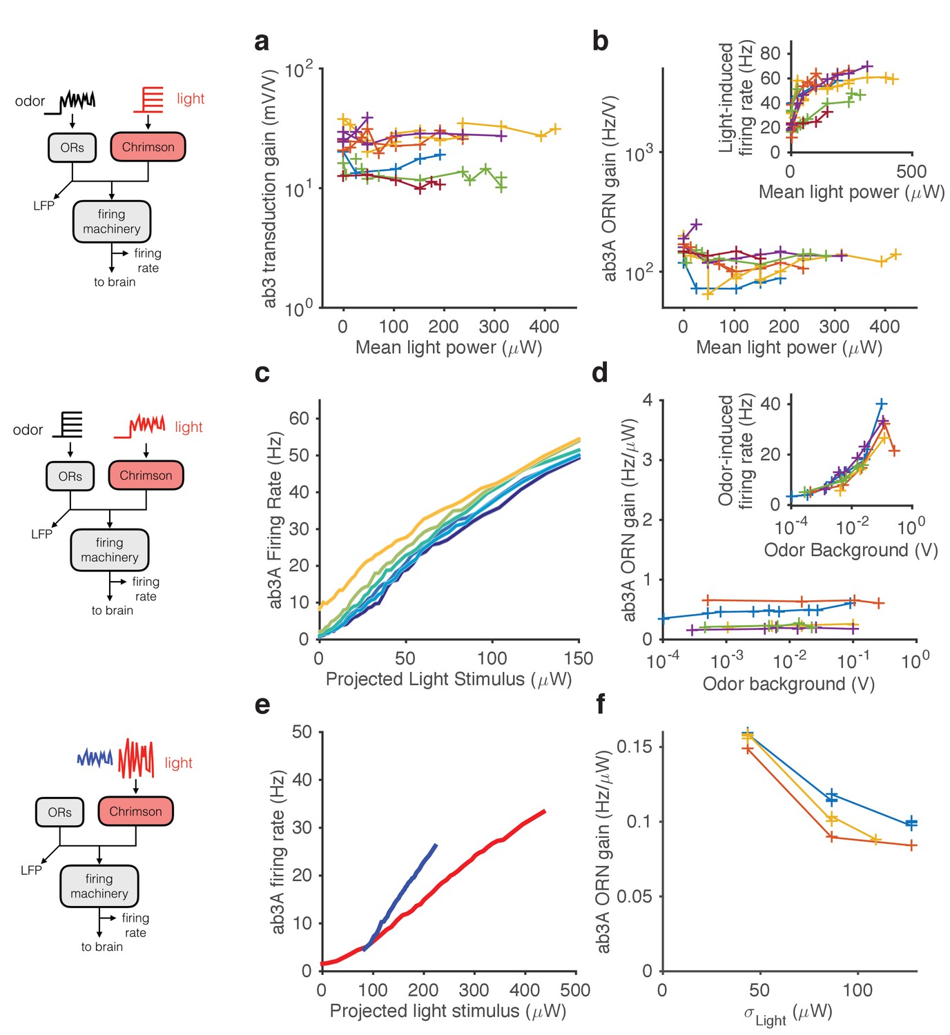
Modularity of gain control revealed by optogenetic stimulation.
ab3A ORNs in w; 22a-GAL4/+; UAS-Chrimson/+ flies can be activated by ethyl acetate odorant or by red light. (a–b) Fluctuating odor foreground and constant light background. (a) Transduction gain to fluctuating odor vs. background light stimulation intensity. (b) Overall ORN gain to fluctuating odor stimulus vs. background light stimulation intensity. (b, inset) ORN firing rate vs. background light intensity. (c–d) Fluctuating light foreground and constant odor background stimulus. (c) Input-output curves to fluctuating light stimulus for increasing background odor (lighter colors indicate larger odor background). (d) ORN gain is invariant with background odor concentration. (d, inset) Odor-induced firing gain vs. background odor concentration. (e–f) Fluctuating light stimulus with different variances. (e) Input-output curves for high (red) and low (blue) variance light stimuli. (f) ORN gain as a function of the standard deviation of the light stimulus. (a–b) n = 75 trials from 13 ORNs. (c–d) n = 64 trials from 5 ORNs. (e–f) n = 21 trials from 3 ORNs. Lines link trials from a single ORN.
Figure 7 with 1 supplement
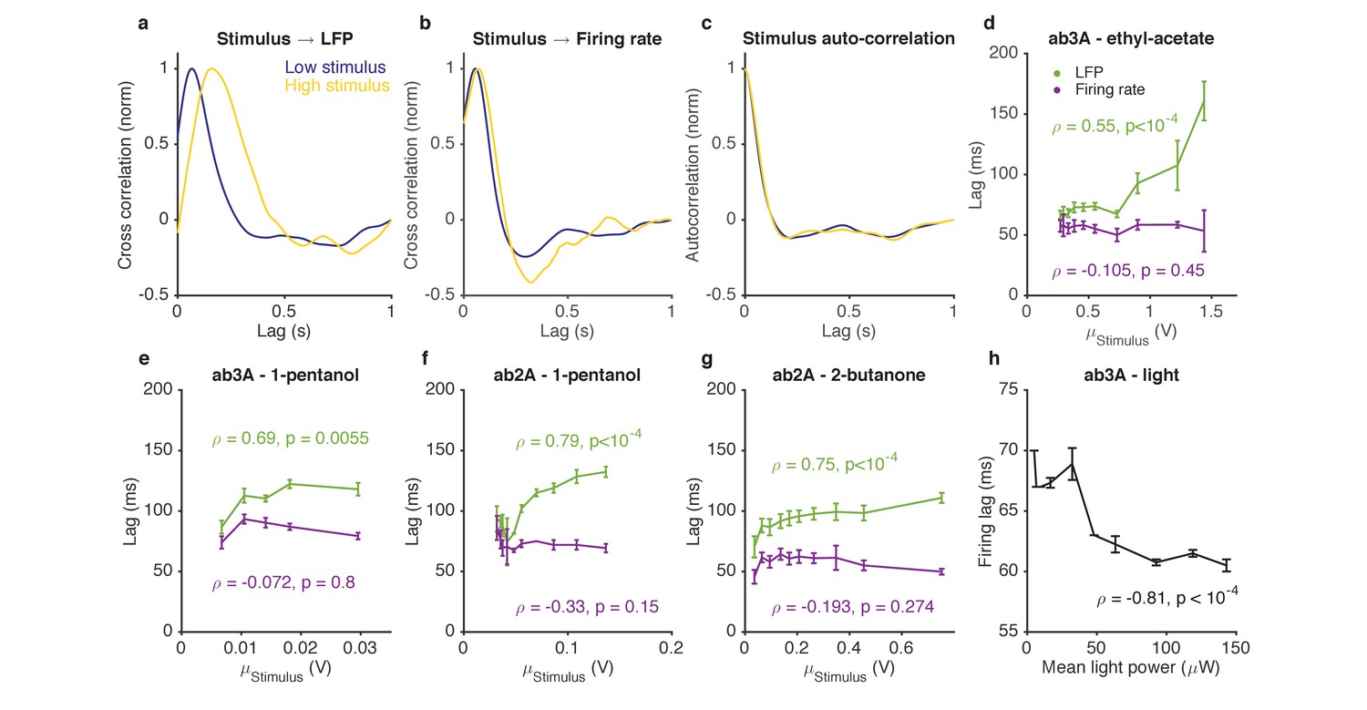
Adaptation to the mean slows down LFP, but not firing rate.
(a–d). Response of ab3A ORNs to Gaussian ethyl acetate stimuli on increasing backgrounds. (a) Cross correlation functions between ethyl acetate stimulus and ab3 LFP responses for low (purple) and high (yellow) background stimuli. (b) Cross correlation functions between ethyl acetate stimulus and ab3A firing rate responses for low (purple) and high (yellow) background stimuli. (c) Stimulus autocorrelation functions for low (purple) and high (yellow) background stimuli. (d–g) LFP and firing rate lags with respect to the stimulus vs. the mean stimulus for various odor-receptor combinations. LFP lags increase with mean stimulus, while firing rate lags do not. (h) Firing lags of ab3A ORNs expressing Chrimson channels vs. applied light power. In (c–g), is the Spearman correlation coefficient, and p is the corresponding p-value.
Figure 7—figure supplement 1
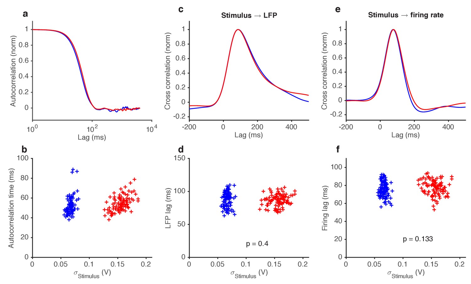
Variance gain control does not change response kinetics.
(a) Stimulus autocorrelation functions, computed during high variance epochs (red) and during low variance epochs (blue). (b) Autocorrelation time (defined as the time the autocorrelation function first drops to 1/e) vs. the standard deviation of the stimulus, for each trial. (c) Cross correlation functions from stimulus to LFP. The cross correlation functions are very similar between high (red) and low (blue) variance epochs. (d) LFP lag with respect to the stimulus, estimated from the location of the peak cross-correlation, vs. standard deviation of the stimulus. No significant change in lag was observed (p=0.4, t-test). (e) Cross correlation functions from stimulus to firing rate. The cross correlation functions are very similar between high (red) and low (blue) variance epochs. (f) Firing rate lag with respect to the stimulus, estimated from the location of the peak cross-correlation, vs. standard deviation of the stimulus. No significant change in lag was observed (p=0.133, t-test).
Figure 8 with 2 supplements
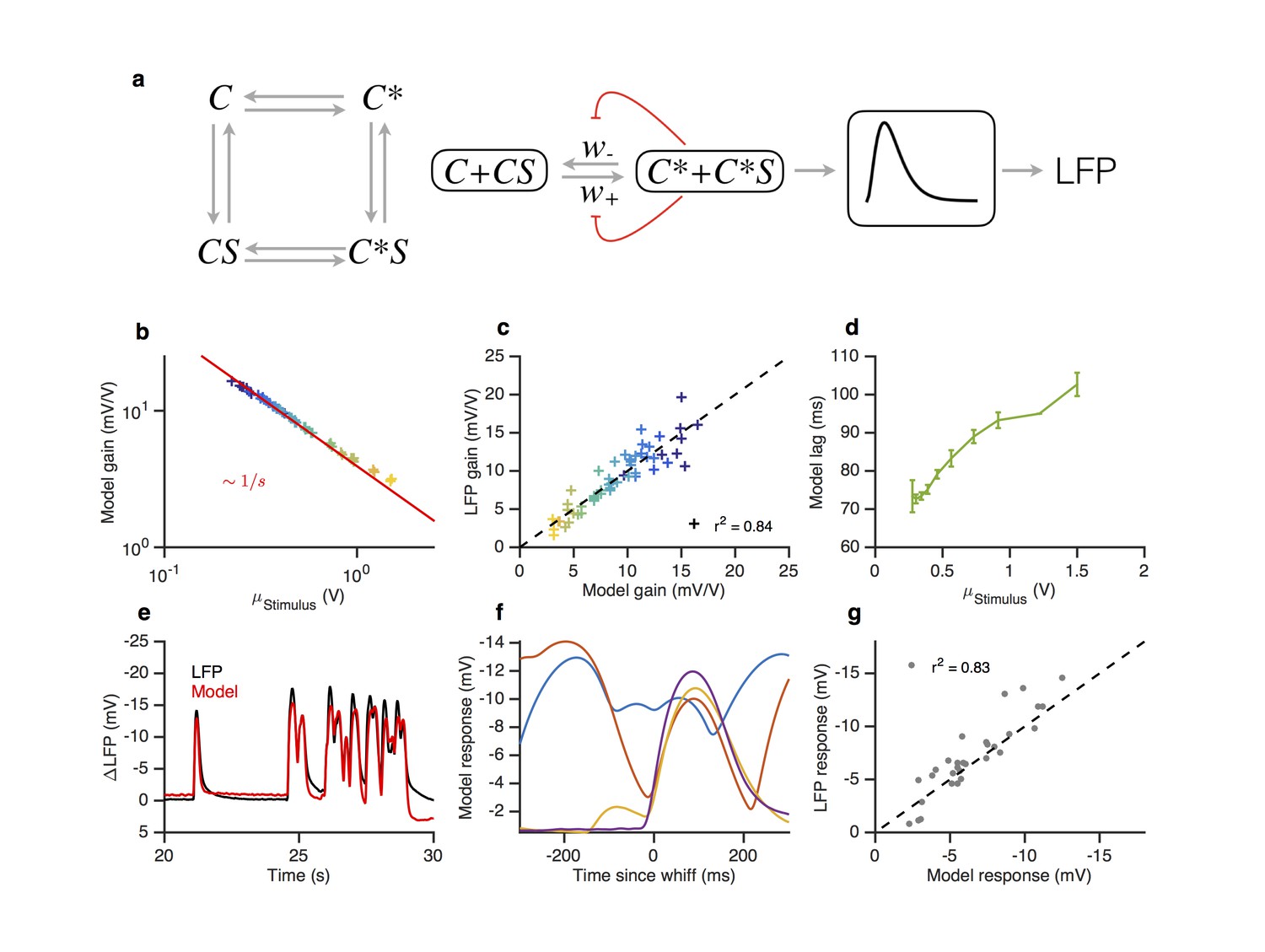
A modified two state receptor model reproduces Weber’s Law and adaptive slowdown in LFP responses.
(a). Or-Orco complexes (C) can be bound or unbound and active or inactive. (b) We assume (un)binding rates are much faster than (in)activation rates. Activity of the complex feeds back onto the free energy difference between active and inactive conformations, which also decreases the activation and inactivation rates of the complex (Equations 1–4). A mono-lobed filter converts receptor activity into LFP signals (Equation 5). We fit the model to Gaussian (Figures 3 and 5) and naturalistic data (Figures 1–2). In these fits, and . (c) Model gain vs. mean stimulus. Red line is the Weber-Fechner prediction (). (c) LFP gain vs. model gain. (e) Model response lag with respect to stimulus vs. mean stimulus. (f) LFP and model responses to naturalistic stimulus. (g) The model reproduces LFP responses to similar-sized whiffs that vary inversely with the size of preceding whiffs. (cf. Figure 2). (h) LFP responses vs. model responses for every whiff in the naturalistic stimulus.
Figure 8—figure supplement 1
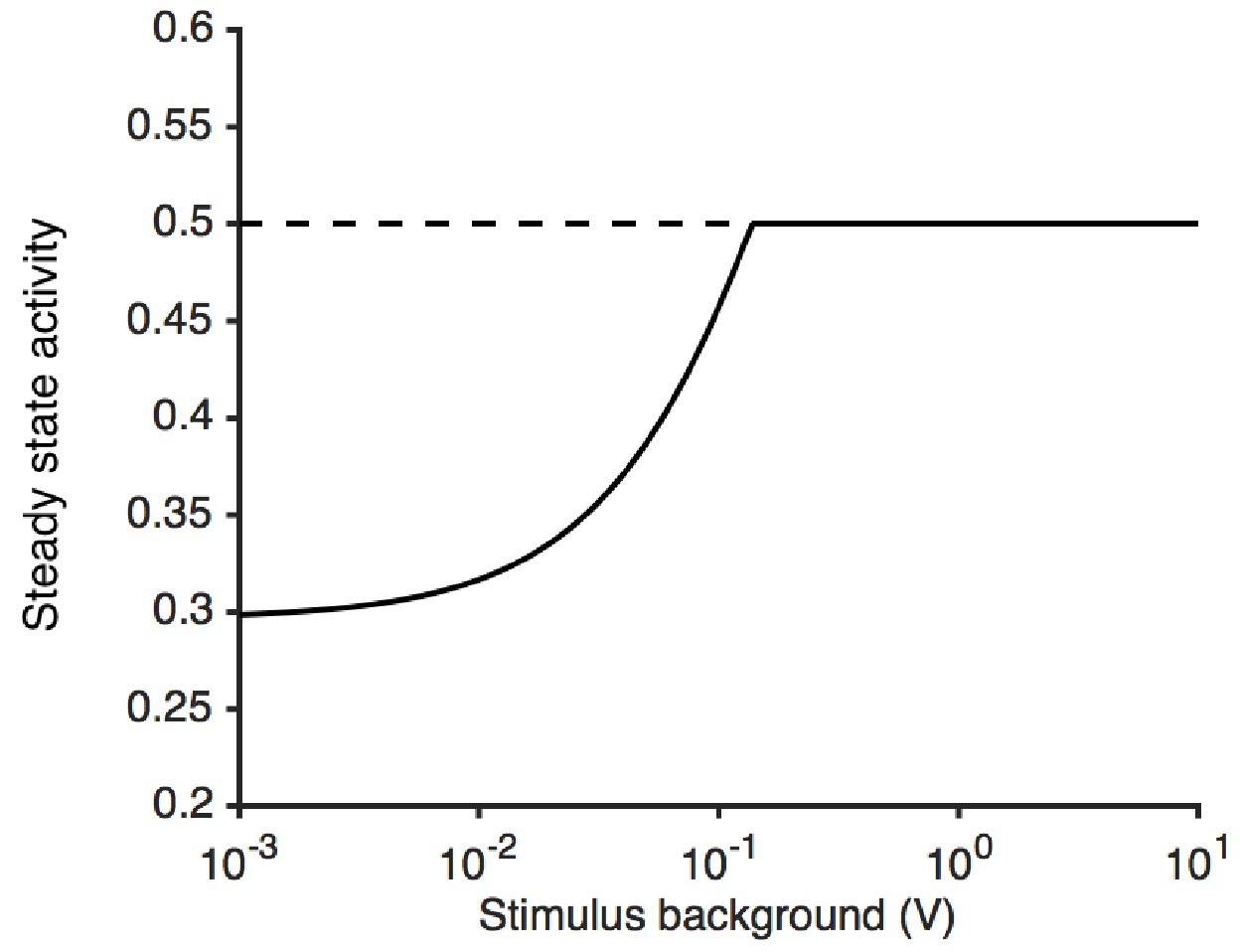
Steady state activity as a function of the stimulus background.
At high stimulus background, the steady state activity of the receptor complex is (here, 1/2). The model is unable to adapt perfectly to lower stimulus backgrounds, since is bounded by . This causes the steady state activity to decrease.
Figure 8—figure supplement 2
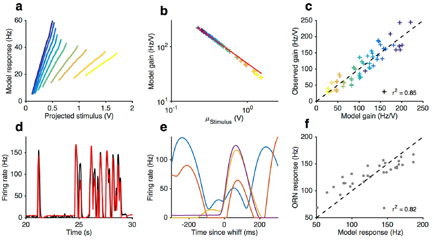
Front-end adaptation followed by a LN model reproduces firing rate responses to Gaussian and naturalistic stimuli.
(a–f) Model from stimulus to firing rate (see Materials and methods) fit to Gaussian and naturalistic stimuli. (a) Model responses vs. projected stimulus with increasing mean stimulus (cf. Figure 3). (b) Model gain vs. mean stimulus. Red line is the Weber-Fechner prediction (). (c) Firing rate gain vs. model gain. (d) Firing rate and model responses to naturalistic stimulus. (e) The model reproduces variation in the firing rate responses to similar-sized whiffs (cf. Figure 2). (f) Firing rate responses vs. model responses for every whiff in the naturalistic stimulus.
Download links
A two-part list of links to download the article, or parts of the article, in various formats.
Downloads (link to download the article as PDF)
Open citations (links to open the citations from this article in various online reference manager services)
Cite this article (links to download the citations from this article in formats compatible with various reference manager tools)
Olfactory receptor neurons use gain control and complementary kinetics to encode intermittent odorant stimuli
eLife 6:e27670.
https://doi.org/10.7554/eLife.27670


