Real-time classification of experience-related ensemble spiking patterns for closed-loop applications
- Neuro-Electronics Research Flanders, Belgium
- KU Leuven, Belgium
- VIB, Belgium
- imec, Belgium
Figures
Figure 1 with 4 supplements
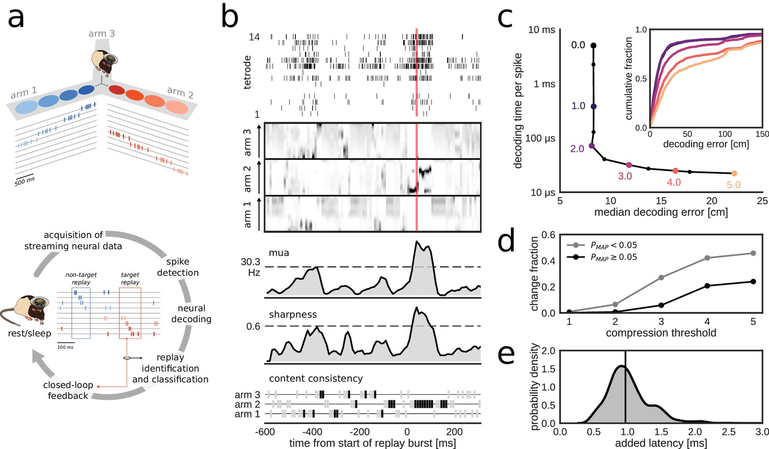
Online decoding and detection of hippocampal replay content for closed-loop scenarios.
(a) Schematic overview of a system for online identification and classification of hippocampal replay content. Top: during the initial active exploration of a 3-arm maze, the relation between the animal’s location and hippocampal population spiking activity is captured in an encoding model for subsequent online neural decoding. Bottom: streaming neural data are processed and analyzed in real-time to detect replay events with user-defined target content. Upon positive detection of a target, closed-loop feedback is provided to the animal within the lifetime of the replay event. (b) Algorithm for online classification of replay content. The top two plots show a raster of all spikes detected on a 14-tetrode array and the corresponding posterior probability distributions for location in the maze generated for non-overlapping 10-ms bins (gray scale maps to 0–0.1 probability). The lower three plots show the internal variables used by the online algorithm to identify and classify replay content. In the bottom plot, gray/black ticks indicate the lack/presence of content consistency across three consecutive bins. Red line: detection triggered when all variables reach preset thresholds (dashed lines for multi-unit activity (MUA) and sharpness, black tick for content consistency). (c) Effect of varying levels of compression on decoding performance and computing time. For the test dataset, compression thresholds in the range [1, 2.5] reduce the decode time to less than 1 ms per spike without affecting the accuracy of decoding the animal’s location in 200 ms time bins during active exploration of a 3-arm maze. Decoding performance was assessed using a 2-fold cross-validation procedure. Inset: full cumulative distributions of decoding error for varying compression thresholds. (d) Effect of compression on posterior probability distributions computed for 10-ms bins in candidate replay bursts. For each level of compression, the plot shows the fraction of posteriors for which the maximum-a-posteriori (MAP) estimate changes to a maze arm different from the no-compression reference condition. Modest compression levels (2) have only a small effect on the MAP estimate, in particular for the most informative posterior distributions with MAP probability > 0.05. (e) Distribution of added latency, that is the time between the acquisition of the most recent 10 ms of raw data and the availability of the posterior probability distribution computed on the same data. Black vertical line represents median latency. Note that online spike extraction, neural decoding and online replay classification add a lag of less than 2 ms.
Figure 1—figure supplement 1

Neural decoding and replay identification over streaming data.
(a) Falcon graph that implemented the real-time processing pipeline of online neural decoding and replay identification and classification. Each box represents a processor node that ran in a separate thread of execution in the central processing unit (CPU). Black arrows indicate ring buffers for data sharing between two connected processors. The first three serially connected processor nodes are responsible respectively for reading the incoming User Datagram Protocol (UDP) packets from the data acquisition system, parsing from the packets the relevant information about the multi-channel signals and dispatching the signals to the downstream processors. The dispatcher processor node streams data to a set of parallel pipelines, each processing data recorded from a different tetrode. Each parallel pipeline has three serially connected processor nodes that are used for digital filtering, spike detection and on-the-fly kernel density estimation of the joint amplitude-position probability density of the spike-sorting-free decoder, which uses the pre-loaded offline-generated encoding models. The likelihoods generated by decoder nodes, each for a different tetrode, are fed into the 'population decoder' node, which produces the final posterior probability distribution of the animal’s real or replayed position. Posterior probability data is streamed to a 'run decoder' node for estimating the animal’s real position and to a 'replay content classifier' node for online detection of a replay content. The output of these nodes are fed to 'file serializer' nodes for data dump (used in post-hoc analysis) and to a 'digital output' node for triggering a closed-loop transistor–transistor logic (TTL) pulse via the dedicated hardware. (b) Flow diagram of the algorithm for replay content identification and classification in streaming data. In the implementation of the 'replay classifier node', an additional check for the sharpness of the most recent 10 ms time bin is performed (threshold was set to). In the software implementation, all criteria are evaluated with an AND condition.
Figure 1—figure supplement 2
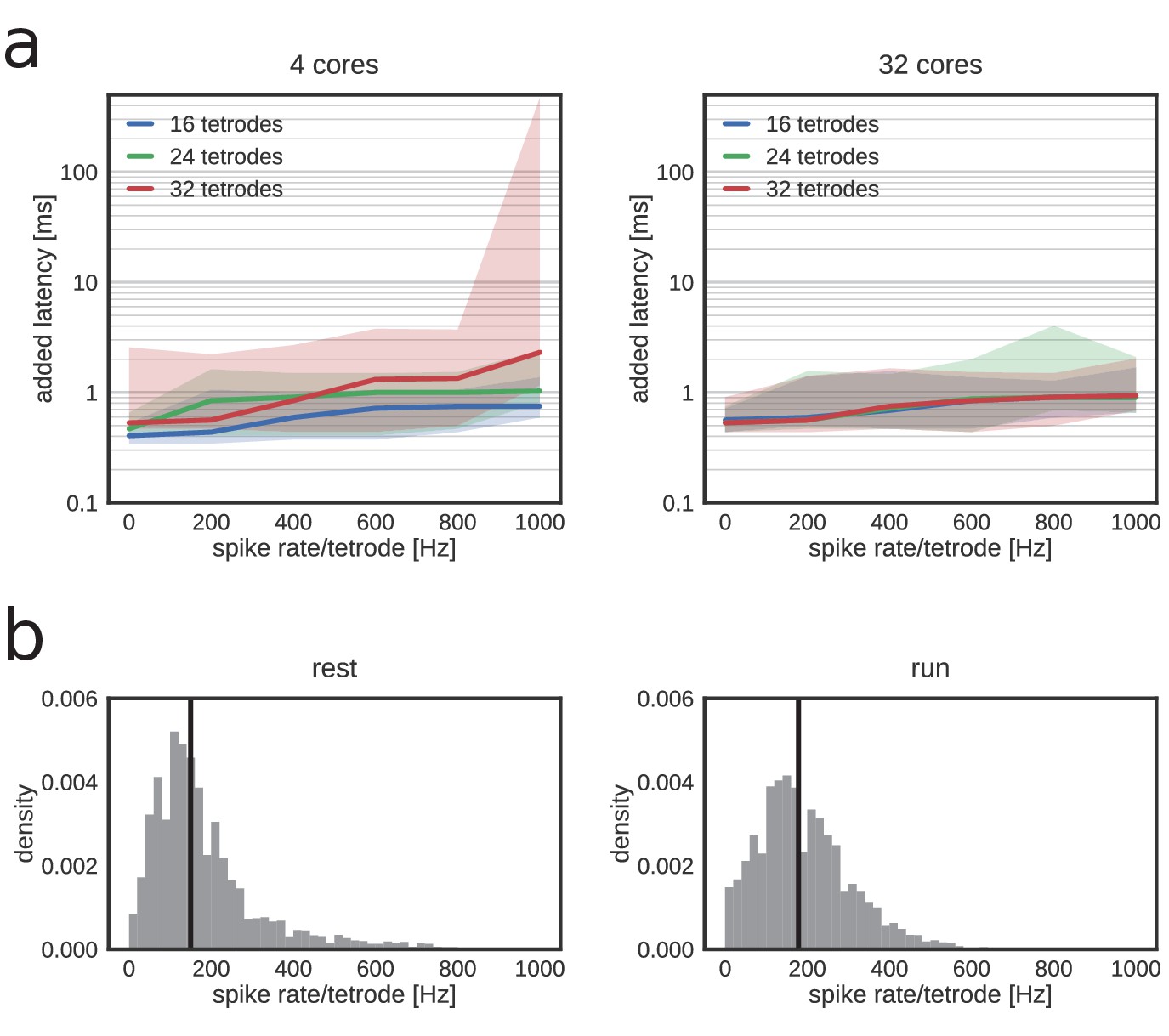
Added latency remains low with higher channel counts and spike rates.
Stress tests used a full decoding pipeline with injected spikes at a predetermined rate. (a) Left: tests performed on a workstation with four physical cores. Thick lines: median. Shaded region: 95% confidence interval (CI). Right: tests performed on workstation with 32 cores. (b) Distribution of actual per-tetrode spike rate in rest (left) and in run (right). Vertical black lines represent median values.
Figure 1—figure supplement 3

Run decoding performance.
(a) Cross-validated decoding performance in RUN1 for all maze arms combined and separately for each arm. Boxes indicate median in-arm error and inter-quartile range. Whiskers indicate most extreme point within 1.5x the inter-quartile range. Horizontal gray line indicates median in-arm error for all arms. Percentages at the top represent the fraction of position estimates that were located in the correct arm. (b) Decoding performance in RUN2 using an encoding model built from spiking data in RUN1.
Figure 1—figure supplement 4
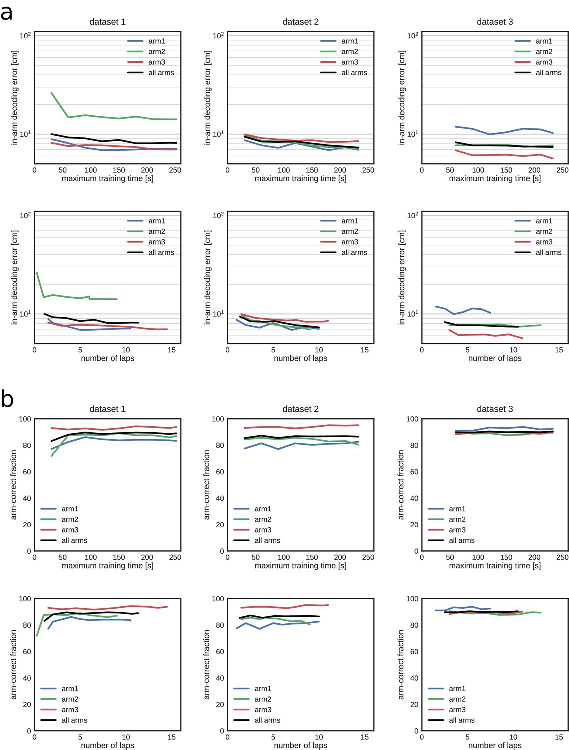
Decoding performance during exploration in all three datasets as a function of the training time and corresponding number of laps used to build the encoding model.
(a) Median in-arm decoding error. Top, REST; bottom, RUN2. (b) Fraction of position estimates that were located in the correct arm. Top, REST; bottom, RUN2.
Figure 2
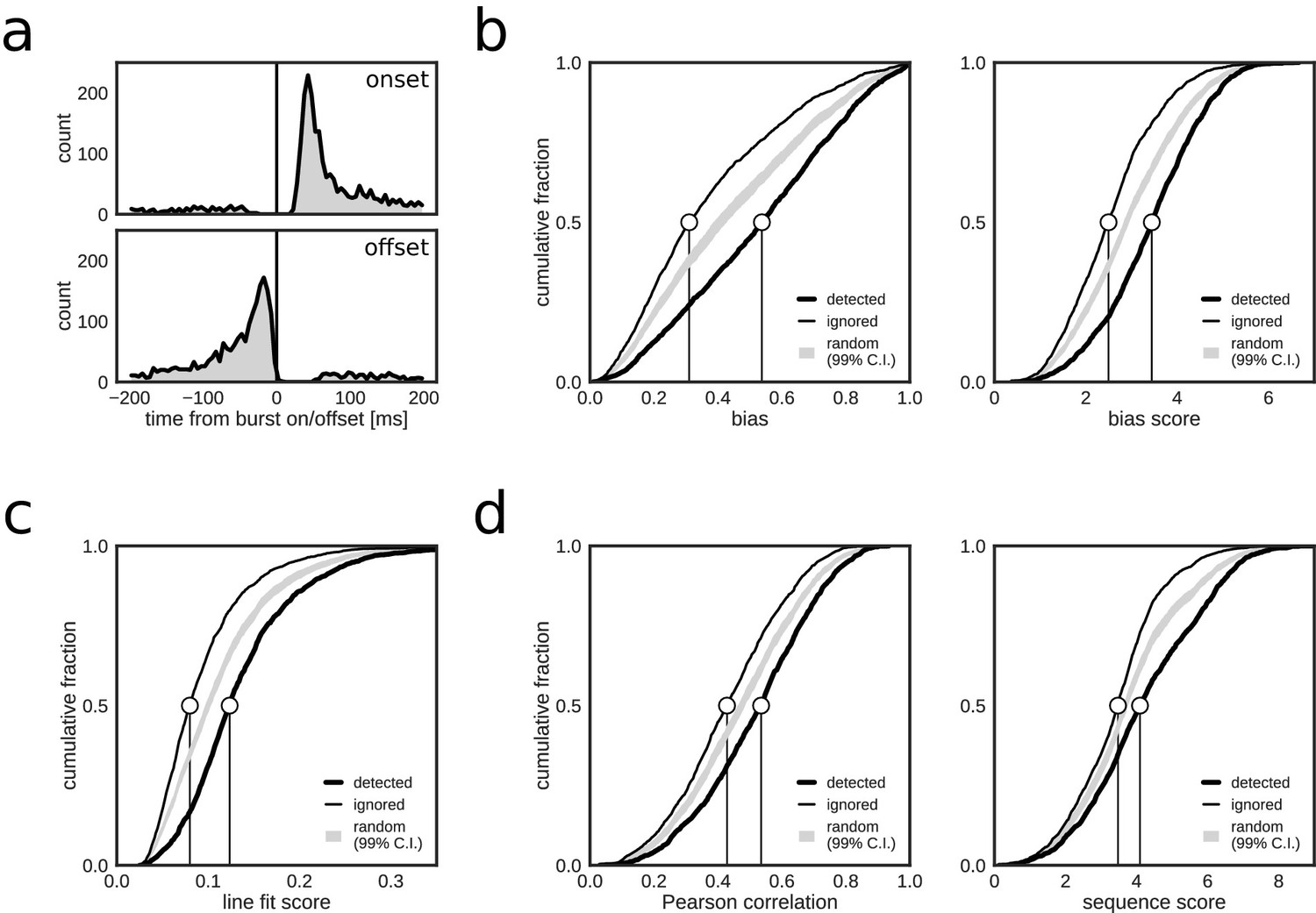
Closed-loop detections correlate with replay content.
(a) Peri-event time histogram of online detections relative to onset (top) and offset (bottom) of reference population bursts. (b–d) Cumulative distributions of different replay content measures for reference bursts that were either flagged online as containing replay (thick line) or that did not trigger an online detection (thin line). Gray shaded area shows the 99% confidence interval (CI) of the cumulative distribution for randomized detections of reference bursts (matched to the average online detection rate). Note that reference bursts that were identified online as replay events are associated with higher values for all of the offline replay content measures.
Figure 3 with 1 supplement
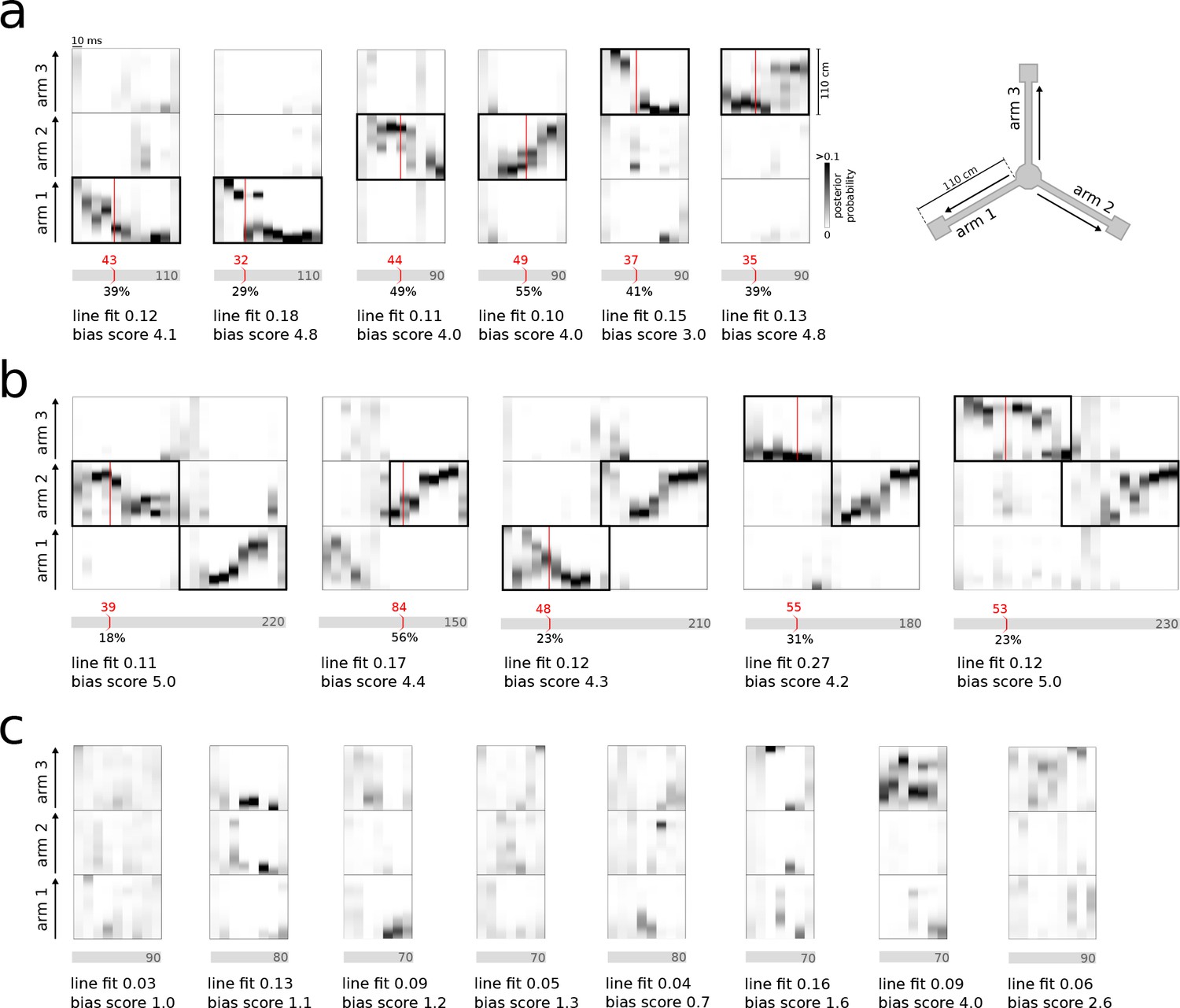
Real-time detection of replay content.
(a) Examples of reference single content replay events that were successfully detected online with correct identification of replay content (vertical red line). The gray bar below each plot represents the total event with duration (in ms) indicated inside the bar. The absolute detection latency from event onset is indicated in red above the bar and the detection latency relative to the duration of the event is indicated below the bar. (b) Similar to (a) but for joint replay events. All examples except the second show online detections triggered by the first replayed arm; the second example shows an online detection that was triggered by a replay of the second arm. (c) Similar to (a) but for reference bursts without replay content that were correctly ignored online.
Figure 3—figure supplement 1

Examples of incorrect online identification of replay.
(a) Examples of false-positive detections. Most incorrect detections were due to spurious matching of the identification criteria in the 30 ms preceding window, without significant reference replay detected offline across the whole population burst. A smaller subset of false-positive detections were due to erroneous decoding of spiking activity (e.g. in the first two examples). (b) Examples of false-negative detections. In the first five events, individual identification criteria were met throughout the population burst but never concurrently. Other false-negative detections were caused by decoding errors (sixth example) or by an online detection that occurred just outside the event (last example).
Figure 4
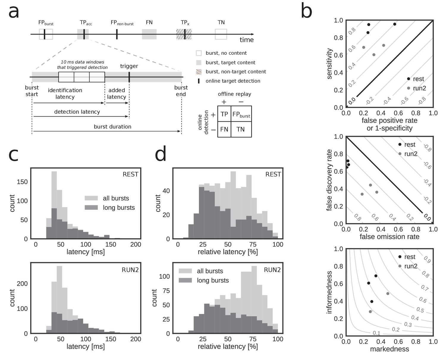
Accurate and rapid online identification of replay bursts.
(a) Schematic overview of the true/false positive/negative classification of online replay detections (top), associated latencies (bottom left) and the confusion matrix used for measuring performance (bottom right). (b) Classification performance measures for all REST (black) and RUN2 (gray) test epochs. Diagonal gray lines in the top and middle plots represent isolines for informedness and markedness measures, respectively. Gray lines in the bottom plot represent isolines for Matthews correlation coefficient. In the bottom graph, two RUN2 epoch values overlap in the lowest gray dot. (c–d) Distribution of absolute (c) and relative (d) online detection latency in REST (top) and RUN2 (bottom) epochs. Light gray: all online detected reference bursts. Dark gray: reference bursts with duration longer than 100 ms.
Figure 5 with 3 supplements
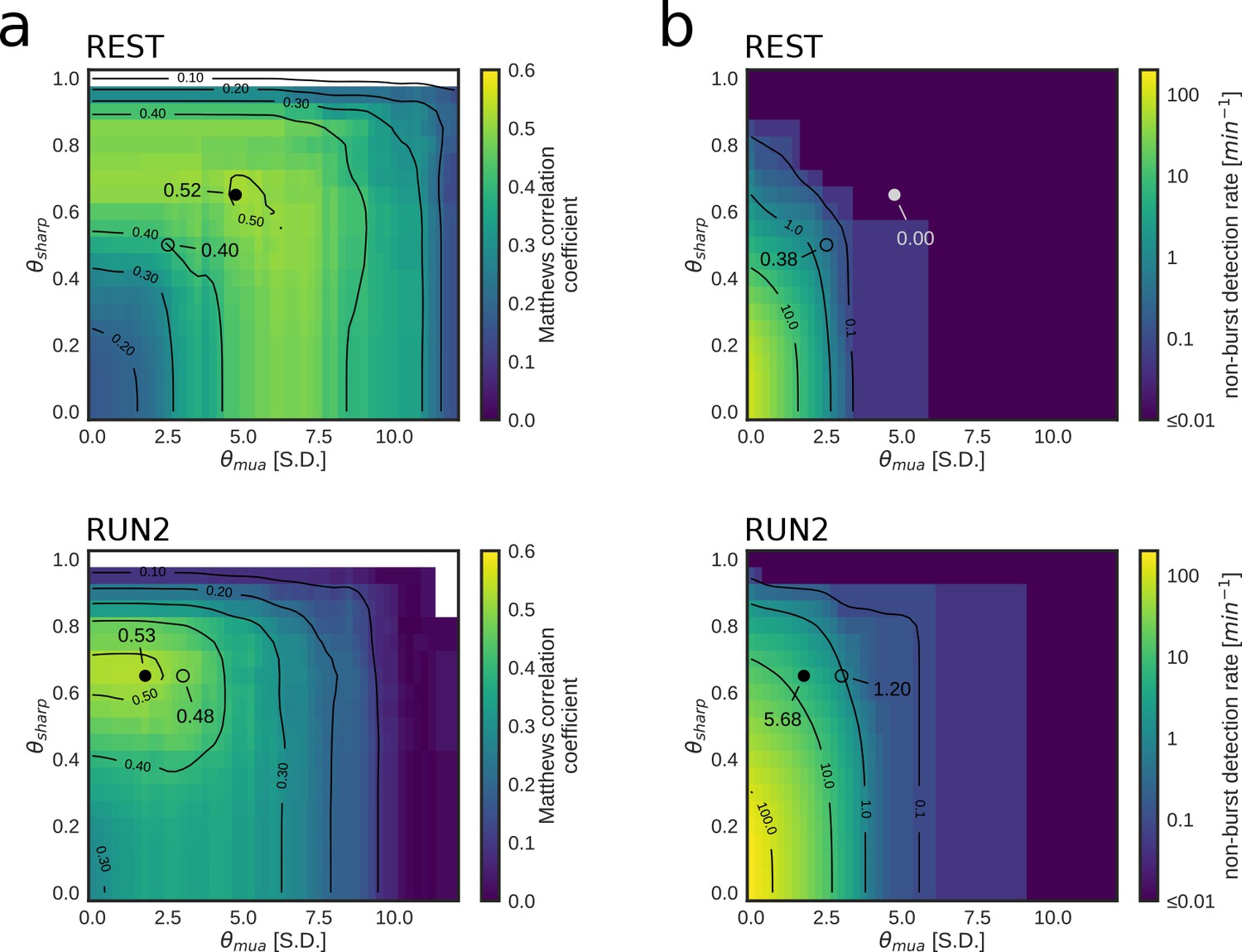
Parameter tuning of online replay detection for optimal detection performance.
(a) Map of the Matthews correlation coefficient for different combinations of values for and of a REST (top) and RUN2 (bottom) epoch; the map was computed using offline playback simulations (dataset 2). Circles indicate the value corresponding to the actual parameters used in the online tests (open circle) and the value corresponding to the set of parameters that maximizes the Matthews correlation coefficient (filled circle). (b) Same as (a) for the non-burst detection rate for different combination of thresholds. Circles indicate the value corresponding to the actual parameters used in the online tests (open circle) and the value corresponding to the set of parameters that maximizes the Matthews correlation coefficient (filled circle).
Figure 5—figure supplement 1

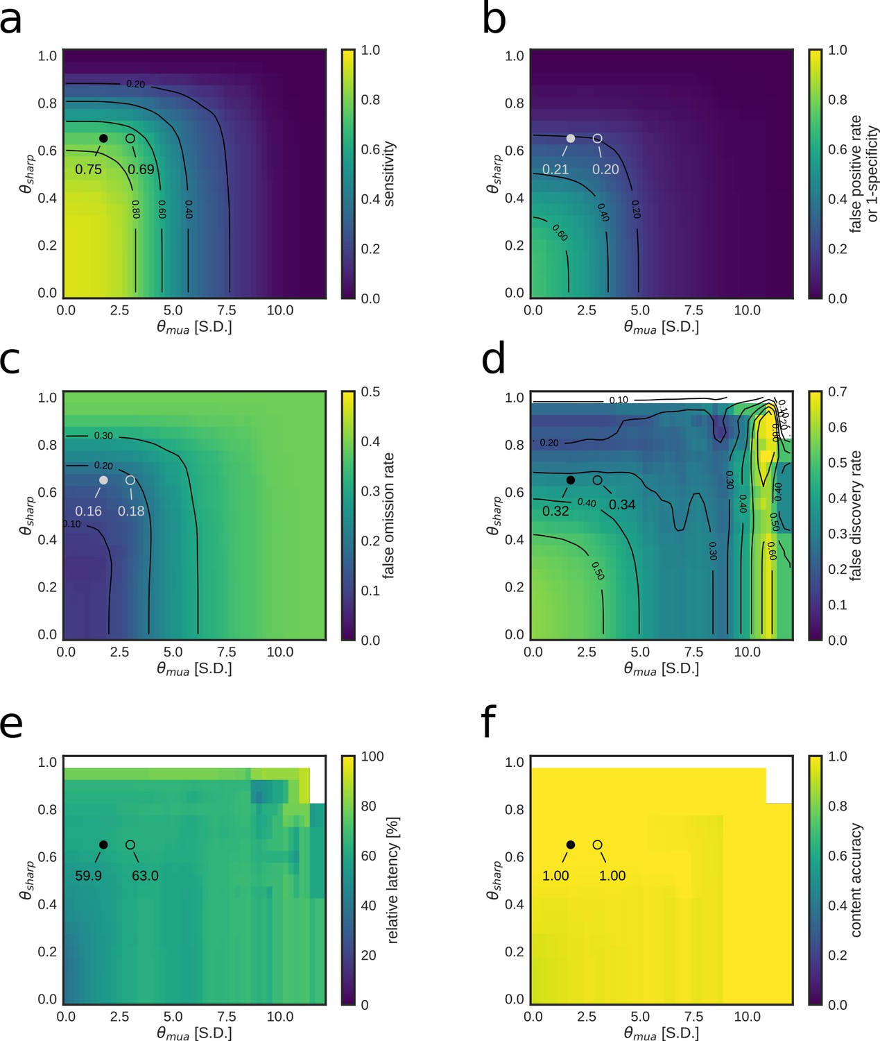
Parameter tuning of the replay content identification algorithm for customized detection performance of a REST epoch.
(a–f) Dependence of online replay detection performance indices on algorithm parameters tested using offline playback simulations with varying combinations of values for and . Circles indicate the value corresponding to the actual parameters used in the online tests (open circle) and the value corresponding to the set of parameters that maximizes the Matthews correlation coefficient (filled circle). Note how lower values of both and improve sensitivity, but negatively affect sspecificity and false discovery rate. On the other hand, median relative latency and content accuracy are not affected by parameter tuning as they depend on other elements of the replay content identification framework.
Figure 5—figure supplement 2
Parameter tuning of the replay content identification algorithm for customized detection performance of a RUN2 epoch.
(a–f) Dependence of online replay detection performance indices on algorithm parameters tested using offline playback simulations with varying combinations of values for and . Circles indicate the value corresponding to the actual parameters used in the online tests (open circle) and the value corresponding to the set of parameters that maximizes the Matthews correlation coefficient (filled circle). Note how lower values of both and improve sensitivity, but negatively affect specificity and false discovery rate. On the other hand, median relative latency and content accuracy are not affected by parameter tuning as they depend on other elements of the replay content identification framework.
Figure 5—figure supplement 3
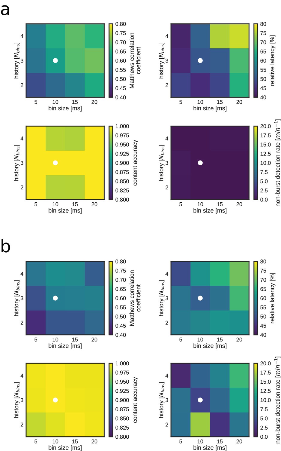
Replay identification performance as a function of time bin size and number of bins (Nbins) for both a REST (a) and RUN2 (b) epoch.
Note that larger Nbins and/or bin size result in both an improved detection performance (i.e. higher Matthews correlation coefficient; top left) and worse detection latency (bottom left). The white dot indicates the combination of bin size and Nbins used for online detections and most offline analyses.
Figure 6 with 2 supplements
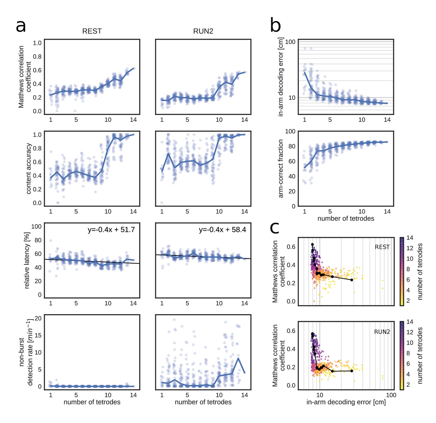
Matthews correlation as a measure of replay identification performance as a function of the number of tetrodes included (up to 50 random selections per tetrode number).
(a) Matthews correlation coefficient, content accuracy, relative detection latency and non-burst detection rate for REST (left) and RUN2 (right). Dots represent individual tests, lines represent the median. (b) Cross-validated RUN1 decoding performance as a function of the number of tetrodes. Top: median in-arm decoding errors. Bottom: fraction arm-correct position estimates. (c) Scatter plot of the relation between median in-arm decoding error and replay detection performance during REST (top) and RUN2 (bottom). Black lines represent the centroid for each color-coded number of tetrodes in vivo.
Figure 6—figure supplement 1
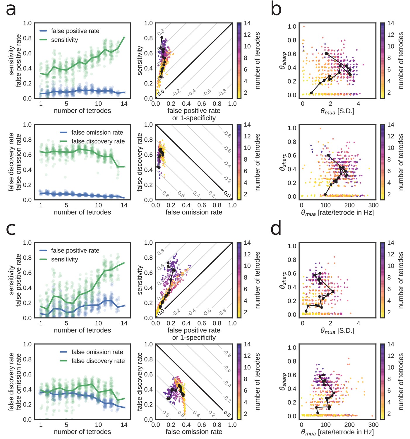
Extended characterization of replay detection performance as a function of number of tetrodes for REST.
(a,b) and RUN2 (c,d). (a,c) Top: sensitivity and false-positive rate. Bottom: false discovery and false omission rates. Diagonal gray lines in scatter plots represent isolines for informedness (top) and markedness (bottom) measures. (b,d) Optimal thresholds with expressed in S.D. (top) or per-tetrode spiking rate (bottom).
Figure 6—figure supplement 2

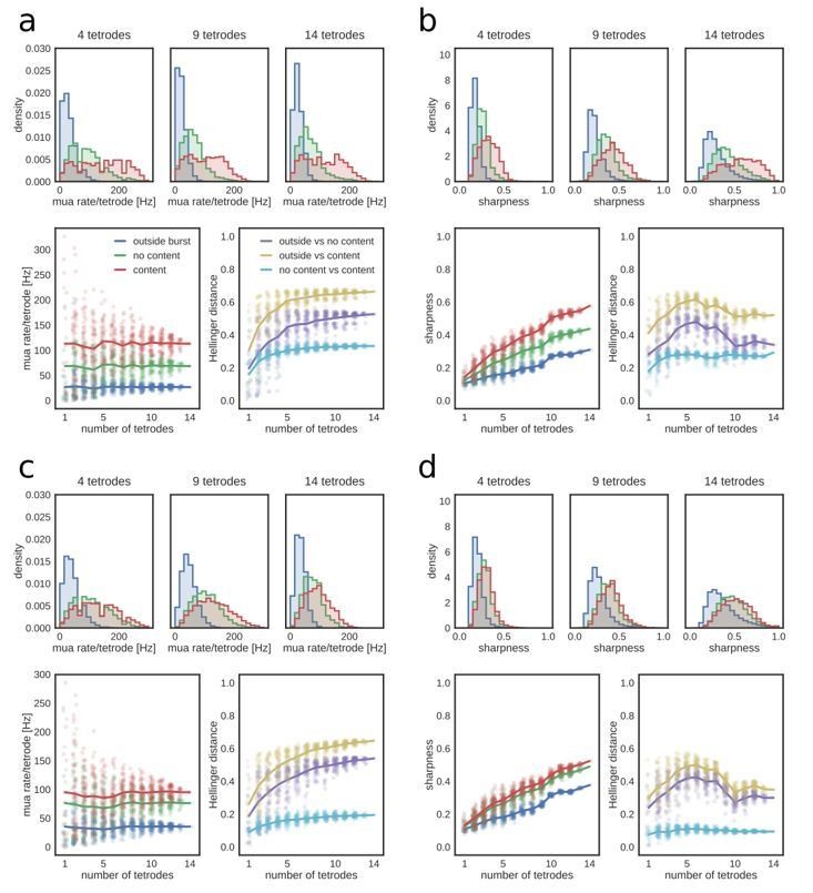
Dependence of MUA and sharpness metrics on the number of tetrodes.
(a) MUA rate per tetrode in REST. Top: example distributions of MUA rate for time bins outside and inside candidate replay bursts (with or without identified replay content) for a subset of 4, 9 and 14 tetrodes. Bottom, left: mean MUA rate as a function of the number of tetrodes. Note that the mean rate remains constant, but the variance increases with fewer tetrodes. Bottom, right: Hellinger distance between MUA rate distributions as a function of the number of tetrodes. (b) Sharpness of posterior probability distributions in REST. Top: example distributions of sharpness values for time bins outside and inside candidate replay bursts (with or without identified replay content) for a subset of 4, 9 and 14 tetrodes. Note shift towards higher sharpness values when more tetrodes are included. Bottom, left: mean sharpness value as a function of the number of tetrodes. Bottom, right: Hellinger distance between sharpness distributions as a function of the number of tetrodes. (c) MUA rate per tetrode in RUN2. Panels as in (a). (d) Sharpness of posterior probability distributions in RUN2. Panels as in (b).
Author response image 1
(a) Example distributions of MUA rate for time bins outside and inside (with or without identified replay content) candidate replay bursts. Rest epoch. (b) Mean MUA rate as a function of the number of tetrodes included. Note that mean rate remains constant, but the variance increases with fewer tetrodes. (c) Hellinger distance between MUA rate distributions as a function of the number of tetrodes included. (d) Optimal θmua threshold as a function of the number of tetrodes included. (a) Example distributions of sharpness values for time bins outside and inside (with or without identified replay content) candidate replay bursts. Rest epoch. Note shift towards higher sharpness values when more tetrodes are included. (b) Mean sharpness value as a function of the number of tetrodes included. (c) Hellinger distance between sharpness distributions as a function of the number of tetrodes included. (d) Optimal θsharp threshold as a function of the number of tetrodes included.
Author response image 2

Decoding performance during exploration in all three datasets as a function of the training time and corresponding number of laps used to build the encoding model.
(a) Median in-arm decoding error. (b) Fraction of position estimates that were located in the correct arm.
Tables
Table 1
Overview of datasets.
https://doi.org/10.7554/eLife.36275.007| Dataset | Epoch | # bursts | Burst rate [Hz] | # replay bursts | # bursts w/joint content | Mean burst duration [ms] |
|---|---|---|---|---|---|---|
| 1 | REST | 297 | 0.40 | 42 | 15 | 107.2 |
| 1 | RUN2 | 663 | 0.56 | 345 | 85 | 94.4 |
| 2 | REST | 537 | 0.43 | 68b) F | 34 | 101.2 |
| 2 | RUN2 | 808 | 0.64 | 315 | 77 | 93.6 |
| 3 | REST | 487 | 0.38 | 134 | 46 | 102.5 |
| 3 | RUN2 | 714 | 0.59 | 334 | 62 | 95.6 |
Table 3
Replay detection performance II.
https://doi.org/10.7554/eLife.36275.012| Dataset | Epoch | Sensitivity | Specificity | False omission rate | False discovery rate | Informedness | Markedness | Correlation |
|---|---|---|---|---|---|---|---|---|
| 1 | REST | 0.95 | 0.74 | 0.01 | 0.65 | 0.69 | 0.34 | 0.49 |
| 1 | RUN2 | 0.60 | 0.68 | 0.35 | 0.36 | 0.29 | 0.29 | 0.29 |
| 2 | REST | 0.86 | 0.75 | 0.02 | 0.72 | 0.61 | 0.26 | 0.40 |
| 2 | RUN2 | 0.69 | 0.80 | 0.18 | 0.34 | 0.49 | 0.48 | 0.48 |
| 3 | REST | 0.95 | 0.44 | 0.03 | 0.68 | 0.40 | 0.30 | 0.34 |
| 3 | RUN2 | 0.71 | 0.57 | 0.28 | 0.44 | 0.28 | 0.28 | 0.28 |
Table 2
Replay detection performance I.
https://doi.org/10.7554/eLife.36275.013| Dataset | Epoch | Out of burst rate [min−1] | Content accuracy | Median absolute latency [ms] | Median relative latency [%] |
|---|---|---|---|---|---|
| 1 | REST | 0.24 | 0.95 | 51.77 | 50.85 |
| 1 | RUN2 | 1.83 | 0.99 | 53.77 | 67.54 |
| 2 | REST | 0.33 | 0.96 | 49.77 | 54.10 |
| 2 | RUN2 | 1.05 | 1.00 | 57.39 | 63.81 |
| 3 | REST | 2.37 | 0.83 | 44.62 | 50.49 |
| 3 | RUN2 | 7.46 | 0.87 | 49.95 | 62.53 |
Table 4
Optimal parameters.
https://doi.org/10.7554/eLife.36275.021| Dataset | Epoch | Live | Live | Optimal | Optimal | Optimal correlation | Correlation live test* | Out of burst rate[min−1] |
|---|---|---|---|---|---|---|---|---|
| 1 | REST | 2.50 | 0.50 | 4.00 | 0.80 | 0.76 | +0.27*** | 0.08 |
| 1 | RUN2 | 3.00 | 0.65 | 0.00 | 0.65 | 0.31 | +0.03 | 28.57 |
| 2 | REST | 2.50 | 0.50 | 4.75 | 0.65 | 0.52 | +0.12** | 0.00 |
| 2 | RUN2 | 3.00 | 0.65 | 1.75 | 0.65 | 0.53 | +0.05 | 5.68 |
| 3 | REST | 2.50 | 0.50 | 5.75 | 0.60 | 0.47 | +0.13** | 0.05 |
| 3 | RUN2 | 3.00 | 0.65 | 1.00 | 0.65 | 0.33 | +0.05 | 30.81 |
-
*Significance: *=p < 0.05, **=p < 0.01, ***=p < 0.001
Additional files
-
Transparent reporting form
- https://doi.org/10.7554/eLife.36275.022
Download links
A two-part list of links to download the article, or parts of the article, in various formats.
Downloads (link to download the article as PDF)
Open citations (links to open the citations from this article in various online reference manager services)
Cite this article (links to download the citations from this article in formats compatible with various reference manager tools)
Real-time classification of experience-related ensemble spiking patterns for closed-loop applications
eLife 7:e36275.
https://doi.org/10.7554/eLife.36275


