Constraints on neural redundancy
- Carnegie Mellon University, United States
- University of Pittsburgh, United States
- Palo Alto Medical Foundation, United States
- Stanford University, United States
Figures
Figure 1 with 1 supplement
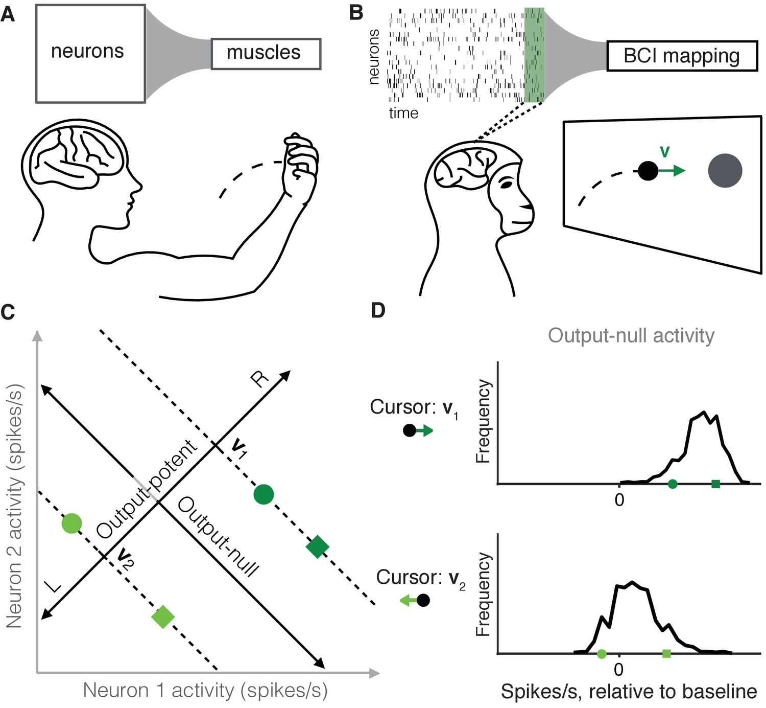
Studying the selection of redundant neural activity.
(A) Millions of neurons in motor cortex drive tens of muscles to move our arms. Thus, different population activity patterns can be redundant, meaning they produce the same muscle activations and movement. (B) In a BCI, the mapping between neural activity and movement is defined by the experimenter. A subject modulates the spiking activity of tens of neurons (green rectangle) to control the 2D velocity () of a cursor on a screen. (C) Example of redundant neural activity in a simplified example where the activity of two neurons (horizontal and vertical axes) drives a 1D cursor velocity (left, L, or right, R). For each of the population activity patterns shown (green squares and circles), the component of the activity along the ‘Output-potent’ axis determines the cursor velocity (e.g. or ), while the position of this activity along the orthogonal axis (‘Output-null’ axis) has no effect on the cursor’s movement. Activity patterns on the same dotted line (e.g. the two dark green patterns) are redundant, because these patterns have the same output-potent activity and produce the same cursor velocity (e.g. ). (D) Example distributions of neural activity along the output-null dimension (corresponding to dotted lines in (C)). Each black trace depicts the density of output-null activity observed over the course of an experiment when the cursor velocity was (top) or (bottom). The output-null activities of the green symbols from (C) are marked for reference. In the actual experiments, there were two output-potent dimensions and eight output-null dimensions. Output-null activity has units of spikes/s, presented relative to the vector of mean activity for each neuron (‘baseline’).
Figure 1—figure supplement 1
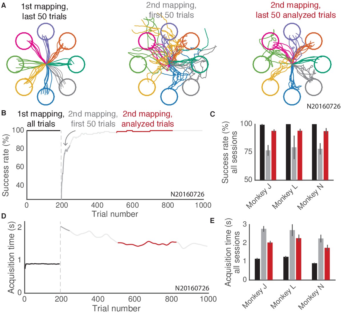
Summary of behavior during the 2D center-out BCI task.
Animals achieved stable control of a computer cursor under two BCI mappings in a 2D center-out task. (A) Cursor traces from 50 consecutive trials during three blocks in an example experiment (N2016726). Cursor traces are colored by the corresponding target on each trial. Cursor positions exceeding a cutoff distance from the workspace center are omitted from view. (B) Success rate during the same example experiment shown in (A), with colors indicating three blocks similar to those shown in (A): all trials under the first mapping (black), the first 50 trials under the second mapping (dark gray), and all analyzed trials under the second mapping (red). Success rates were smoothed using a 100-trial moving window. (C) Average success rate across all sessions for each of three animals, during the three blocks highlighted in (B). Error bars depict mean SE. (D) Same conventions as (B), for target acquisition time. Acquisition times were computed during successful trials only. For each session, for analysis we identified a consecutive block of at least 100 trials that showed both substantial learning of the second mapping and consistent behavior. Trials with substantial learning were identified by thresholding the smoothed acquisition times shown here (see Materials and methods). Only correct trials within this block were analyzed. (E) Same conventions as (C), for acquisition time.
Figure 2
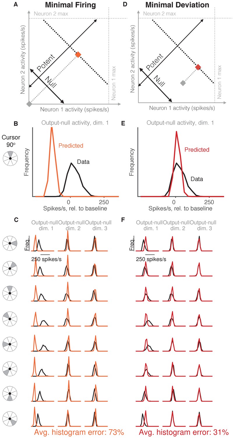
Minimal firing hypotheses.
(A) Minimal Firing hypothesis: Given a particular output-potent activity (i.e. activity is constrained to black dotted line), subject selects the activity pattern (orange square) that requires the fewest spikes (i.e. nearest the gray square). (B) Distribution of observed output-null activity (‘Data’, in black) and activity predicted by the Minimal Firing hypothesis (‘Predicted’, in orange), in the first output-null dimension for upwards cursor movements. For this visualization, we applied PCA to the observed output-null activity to display the dimensions ordered by the amount of shared variance, with only the first of those dimensions shown here. The range of activity (e.g. 150 spikes/s) appears larger than that expected for a single neuron because the range tends to increase with the number of neural units contributing to that dimension. Session L20131218. (C) Distributions of observed and predicted output-null activity as in (B), for time steps when the cursor was moving in eight different directions (rows), in three (of eight) output-null dimensions explaining the most output-null variance (columns). (D) Minimal Deviation hypothesis: Given a particular output-potent activity, subject selects the activity pattern (red square) nearest a fixed population activity pattern chosen for each session by cross-validation (gray square). (E–F) Same conventions as in (B–C) for the Minimal Deviation hypothesis.
-
Figure 2—source data 1
Histograms of predictions and data, as depicted in Figure 2B–C and Figure 2E–F.
- https://doi.org/10.7554/eLife.36774.006
Figure 3
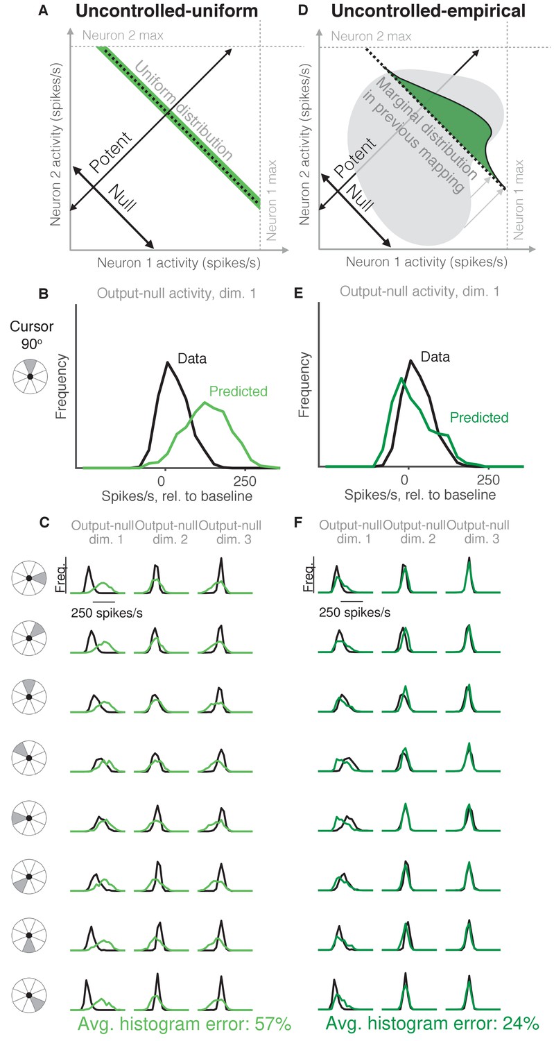
Uncontrolled hypotheses.
(A) Uncontrolled-uniform hypothesis: Given a particular output-potent activity, subject selects any activity within the physiological range (dark green), sampled from a uniform distribution. (B–C) Distributions of output-null activity observed and predicted by the Uncontrolled-uniform hypothesis; same conventions as in Figure 2. The predicted distributions appear mound-shaped rather than uniform because we applied PCA to display the dimensions of output-null activity with the most shared variance (see Materials and methods). The range of activity increases with the number of neural units. Session L20131218. (D) Uncontrolled-empirical hypothesis: Subject selects output-null activity from the distribution of all output-null activity produced at any time while subjects used a different BCI mapping. (E–F) Same conventions as in (B–C) for the Uncontrolled-empirical hypothesis.
-
Figure 3—source data 1
Histograms of predictions and data, as depicted in Figure 3B–C and Figure 3E–F.
- https://doi.org/10.7554/eLife.36774.008
Figure 4
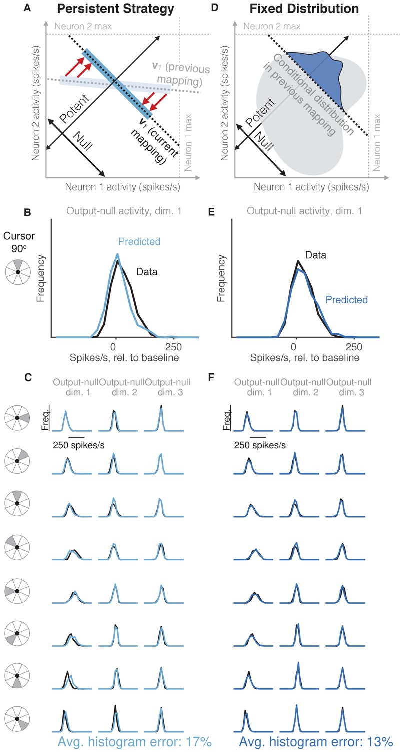
Task-transfer hypotheses.
(A) Persistent Strategy hypothesis: Given a particular output-potent activity, subject selects an activity pattern appropriate under a different mapping (light blue rectangle), and corrects its output-potent component (red arrows) so as to produce the desired output-potent value under the current mapping (darker blue rectangle). (B–C) Distributions of output-null activity observed and predicted by the Persistent Strategy hypothesis; same conventions as in Figure 2. The range of activity increases with the number of neural units. Session L20131218. (D) Fixed Distribution hypothesis: Given a particular output-potent activity, subject selects from the output-null activity patterns that were observed concurrently with this output-potent activity while controlling a different mapping. Different patterns are selected with the same frequencies as they were under the previous mapping. (E–F) Same conventions as in (B–C) for the Fixed Distribution hypothesis.
-
Figure 4—source data 1
Histograms of predictions and data, as depicted in Figure 4B–C and Figure 4E–F.
- https://doi.org/10.7554/eLife.36774.010
Figure 5 with 4 supplements

Fixed Distribution hypothesis best predicts output-null activity.
Boxes depict the 25th, 50th, and 75th percentile of errors observed across sessions for all animals combined. Whiskers extend to cover approximately 99.3% of the data. Gray boxes depict the error floor across sessions (mean ± s.d.), estimated using half of the observed output-null activity to estimate the histogram, mean, and covariance of the other half (see Materials and methods). Asterisks depict a significant difference between errors of Fixed Distribution and other hypotheses for a one-sided Wilcoxon signed rank test at the (***) level. (A) Error in predicted histograms of output-null activity. For each session, histogram error was averaged across all output-null dimensions and cursor directions. Average histogram error floor was 6.7% ± 1.9% (mean ± s.d., also shown in gray). (B) Error in predicted mean of output-null activity. For each session, mean error was averaged across all cursor directions, where the mean is an 8D vector of the average activity in each output-null dimension. Average mean error floor was 6.9 ± 2.5 spikes/s (mean ± s.d., also shown in gray). (C) Error in predicted covariance of output-null activity. For each session, covariance error was averaged across all cursor directions. Average covariance error floor was 1.0 ± 0.3 (mean ± s.d., also shown in gray).
-
Figure 5—source data 1
Histogram, mean, and covariance errors of all hypotheses for all sessions, as depicted in Figure 5 and Figure 5—figure supplement 1.
- https://doi.org/10.7554/eLife.36774.016
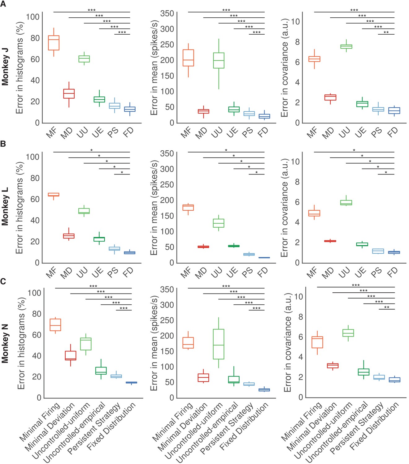
Figure 5—figure supplement 1
Results for each animal.
Fixed Distribution hypothesis best predicts observed output-null activity for each animal. (A) Monkey J. (B) Monkey L. (C) Monkey N. Same conventions as Figure 5. Asterisks denote a significance level of (*), (**), and (***).
Figure 5—figure supplement 2

Results when predicting output-null activity during first mapping.
Predicting output-null activity produced during the first mapping using activity observed during the second mapping. Throughout this work, we predict the output-null activity recorded while subjects used the second BCI mapping, and hypotheses can use activity recorded during use of the first BCI mapping to make their predictions. However, most of the hypotheses do not depend on the order in which the two mappings were presented to the subjects. Here we predict the output-null component of the activity recorded during use of the first BCI mapping, and hypotheses can use activity recorded under the second BCI mapping to make their predictions. Same conventions as Figure 5.
Figure 5—figure supplement 3

Results when not using animals’ internal model to define the output-null dimensions.
Predicting output-null activity without using animal’s internal model (IME) to define the output-null dimensions. Same conventions as Figure 5. Asterisks denote a significance level of (*), (**), and (***). ‘n.s.’ is not significant.
Figure 5—figure supplement 4
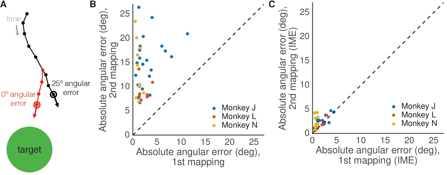
Identifying the animal’s internal model to define the output-null dimensions.
Identifying the animal’s internal model of the BCI mapping. (A) BCI cursor trajectory (black) for an example trial during the second mapping. At each time step, the subject takes its most recent visual feedback (where red whisker touches black trajectory) and propagates it forward in time (red whisker) using an internal model and neural activity produced in the recent past. This yields the subject’s internal estimate of the current cursor position (red open circle), which is different from the actual BCI cursor position (black open circle). At this time step, the cursor movement according to the internal model (red arrow) points more directly to the target (green circle) than the actual BCI cursor movement (black arrow). Each dot indicates a 45 ms time step. (B) Average absolute angular cursor error (in degrees) for each session based on the actual BCI cursor movements (analogous to black arrow in (A)). Angular errors during stable control of the second mapping were larger than the angular errors during control of the first mapping. (C) Average absolute angular cursor error (in degrees) for each session based on IME (analogous to red arrow in (A)). When viewed through animals’ internal estimates of the BCI, angular errors during control of the first and second mapping were similar.
Figure 6 with 2 supplements
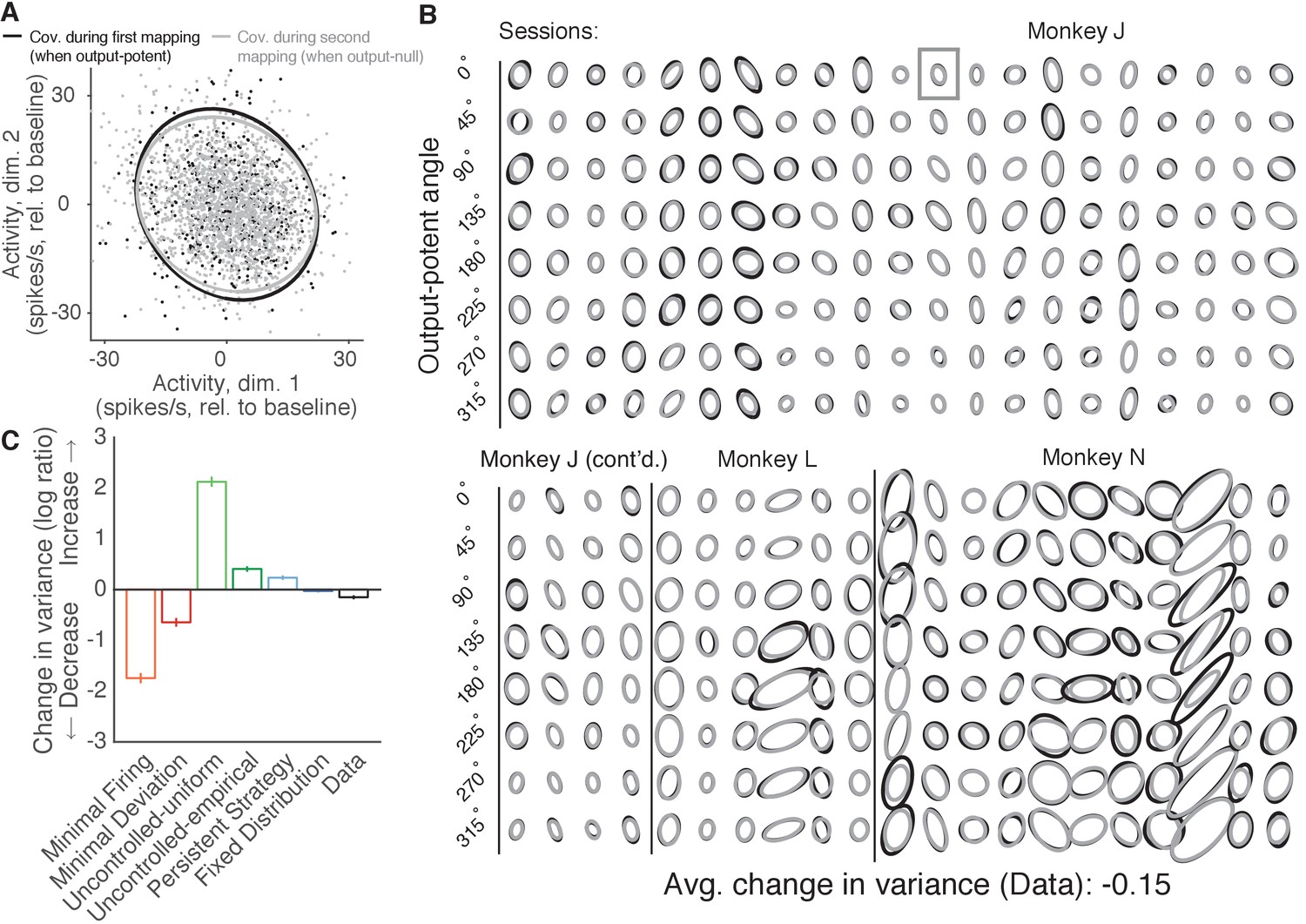
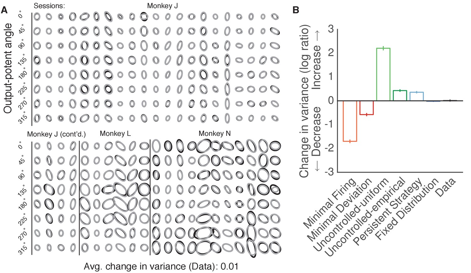
Variance of neural activity in dimensions that become output-null.
(A) Observed activity from a representative session in the 2D subspace in which activity was output-potent under the first mapping and output-null under the second mapping. Activity recorded during use of the first mapping (black points) was output-potent while activity recorded during use of the second mapping (gray points) was output-null. The covariances during the first and second mapping (black and gray ellipses, respectively) are depicted as the 95% contours of a Gaussian density fit to the activity. Session J20120403, for all time steps when the activity would have moved the cursor to the right under the second mapping. (B) Covariance ellipses for all sessions and eight different cursor movement angles. Same conventions as in (A). Ellipses shown in (A) indicated by gray box. (C) Change in variance of neural activity in the same subspace as in (A), for the activity observed (‘Data’) and predicted by each hypothesis. Height of bars depicts the average change in variance across sessions (mean ± 2 SE).
-
Figure 6—source data 1
Observed and predicted change in covariance across sessions, as depicted in Figure 6C.
- https://doi.org/10.7554/eLife.36774.020
Figure 6—figure supplement 1
Variance of neural activity did not change in the dimensions that became output-potent.
Variance of neural activity in dimensions that became output-potent. We repeated the analyses shown in Figure 6 on the predictions of output-null activity produced during the first mapping using activity observed during the second mapping (shown in Figure 5—figure supplement 2). This analysis amounts to assessing the change in variance in dimensions that were output-null during the first mapping and output-potent during the second mapping. Same conventions as Figure 6B–C.
Figure 6—figure supplement 2
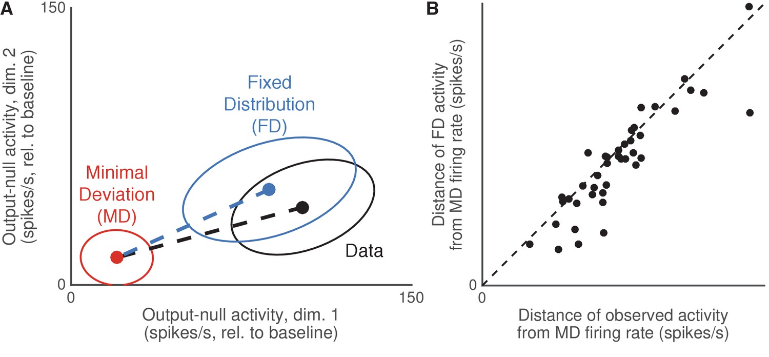
Decrease in variance was not accompanied by the mean activity moving toward predictions of minimal energy hypotheses.
Output-null activity was not closer to the mean predicted by Minimal Deviation than expected under Fixed Distribution. (A) Determining whether the observed mean output-null activity (‘Data’) was closer to the Minimal Deviation (‘MD’) prediction than expected under Fixed Distribution (‘FD’). Dots and ellipses indicate the mean and covariance of output-null activity observed (black), predicted by Fixed Distribution (blue), and predicted by Minimal Deviation (red), for all time steps from session J20160714 corresponding to the same cursor movement, in the first two of eight output-null dimensions. Similar to Figure 6, the observed covariance (black ellipse) is slightly smaller than that of Fixed Distribution (blue), suggesting the observed covariance is moving in the direction of the small covariance expected under Minimal Deviation (red). Do we see a similar trend in the mean activity, where the observed mean activity is closer to the Minimal Deviation mean than expected under Fixed Distribution? We can assess this by comparing the lengths of the dotted lines, which indicate the distances of the mean activity observed (black) and predicted by Fixed Distribution (blue) from the mean predicted by Minimal Deviation. (B) Distance of the observed and predicted output-null activity from the activity predicted by Minimal Deviation. Each dot indicates the average distance of the output-null activity observed (horizontal axis) and predicted by Fixed Distribution (vertical axis, ‘FD’) from the Minimal Deviation (‘MD’) in a session. For each cursor direction, the distance was computed as the norm of the difference between the mean 8D output-null activity (predicted or observed) from the mean activity predicted by MD, similar to (A). Session distances were the average distances across all cursor directions. Most points lie below the diagonal, suggesting that the observed output-null activity was not closer to the MD predictions than expected under Fixed Distribution. Results were similar when comparing distances to the means predicted by Minimal Firing instead of Minimal Deviation.
Appendix 1—figure 1
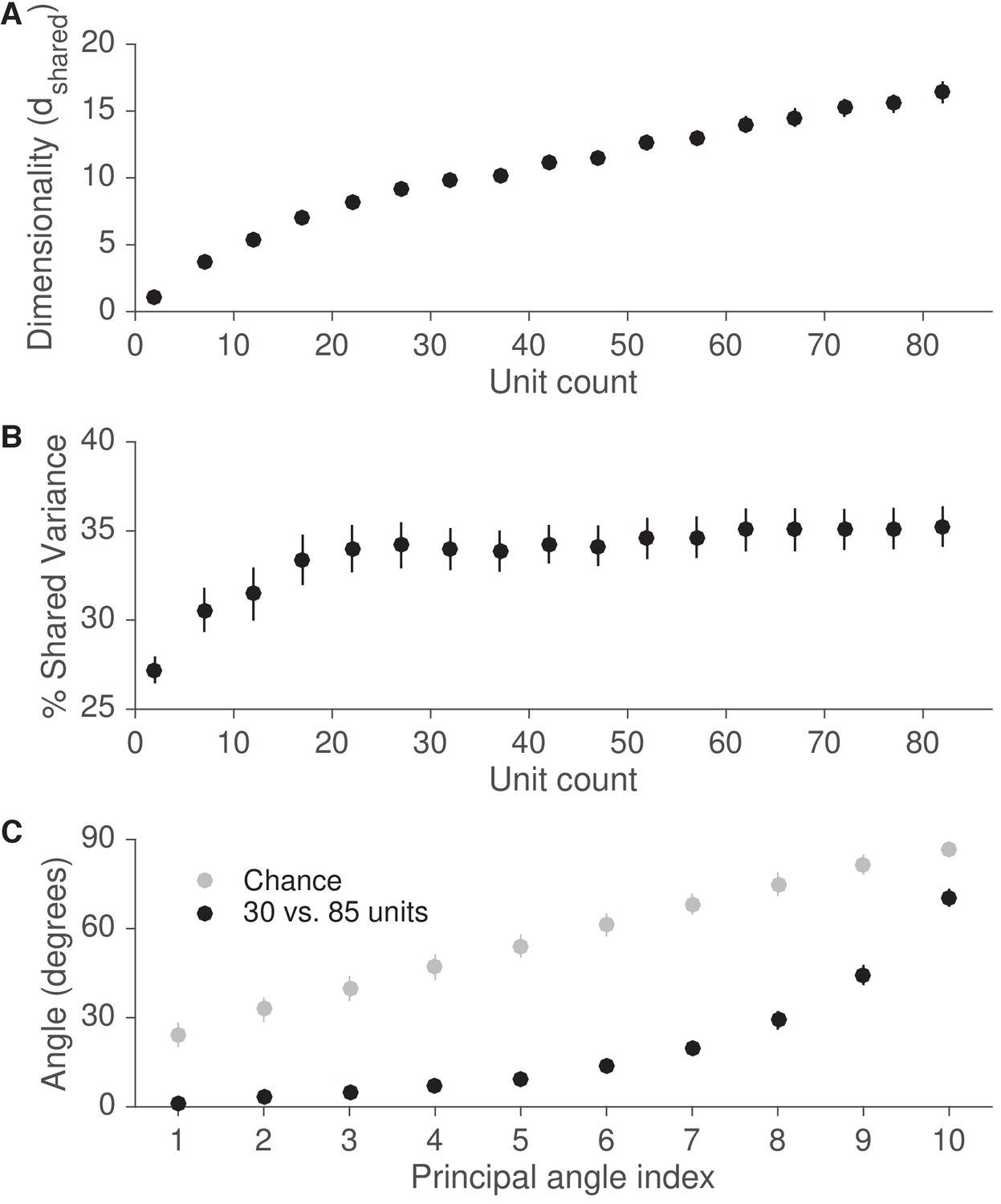
Recording from more units is likely to reveal an intrinsic manifold similar to that identified in this study.
(A) We assessed the dimensionality () of population activity after applying factor analysis to varying numbers of units from each session. Dimensionality is defined as the number of factors needed to explain 95% of the shared variance. Dimensionality increased with the number of units. Error bars depict mean SE, across sessions. (B) We also computed the percentage of each neural unit’s activity variance that was shared with other recorded units (% shared variance). The % shared variance is based on the same factor analysis models identified in (A). The % shared variance initially increased with the number of units, then reached an asymptote, such that the % shared variance was similar with 30 and 85 units. Error bars depict mean SE, across sessions. (C) We next measured the principal angles between the modes identified by factor analysis using 30 units with those identified using 85 units. Modes are defined as the eigenvectors of the shared covariance matrices corresponding to units from the 30-unit set. The small principal angles between modes identified using 30 and 85 units indicate that the dominant modes remained largely unchanged when using more units. Gray points represent principal angles between random 30-dimensional vectors. Error bars for black points depict mean SE, across sessions, while error bars for gray points depict mean s.d.
Additional files
-
Supplementary file 1
Table of statistical tests.
- https://doi.org/10.7554/eLife.36774.021
-
Transparent reporting form
- https://doi.org/10.7554/eLife.36774.022
Download links
A two-part list of links to download the article, or parts of the article, in various formats.
Downloads (link to download the article as PDF)
Open citations (links to open the citations from this article in various online reference manager services)
Cite this article (links to download the citations from this article in formats compatible with various reference manager tools)
Constraints on neural redundancy
eLife 7:e36774.
https://doi.org/10.7554/eLife.36774


