Neuronal morphologies built for reliable physiology in a rhythmic motor circuit
- Brandeis University, United States
- Marine Biological Laboratories, United States
Figures
Figure 1 with 2 supplements

Electrotonus in cable models with diverse passive properties and geometries.
(A) Illustration of the complete matrix of cable model geometries assessed in the computational simulation. Proximal diameters (d0) ranged between 0.5–20 µm and distal diameters (d1) ranged between 0.5–10 µm, yielding 20 different geometries spanning from fine, uniform-diameter cylinders to immensely tapered cables. Shaded areas indicate geometries consistent with vertebrate neocortical and hippocampal pyramidal neuron dendrites (gray) and neurites of STG neurons (blue). (B) Top: illustration depicting simulated measurement of the effective electrotonic length constant (λeffective) in a classic cable model with a uniform 0.5 µm-diameter (Rm = 10000 Ω*cm2 and Ra = 100 Ω*cm). An inhibitory potential (Erev = −75 mV, 𝜏 = 70 ms, gmax = 10 nS) was evoked at a distal site (gray circle) and recorded (blue traces) at increasing distances from the site of activation (0, 100, 250, 400, 550, 700, 850 µm). Bottom: Plot depicts the amplitude of the evoked inhibitory potential measured at increasing distances from the activation site (at 0 µm; gray dashed line), illustrating electrotonic decrement of propagating voltage signal. λeffective (315 µm) was calculated as the distance (black dashed line) at which the recorded potential was 37% of the maximal amplitude at the activation site (purple dashed line). (C) λeffective for cables with fixed, narrow, uniform diameter (as in B; d0 = d1=0.5 µm) and varying passive properties. λeffective is plotted as a function of axial resistivity (Ra in Ω*cm) for cables with different specific membrane resistivities (Rm in Ω*cm2; plotted in different colors). (D) Top: illustration showing simulated measurement of λeffective (as in B, Top) in a cable model with geometry reminiscent of an STG neurite (d0 = 20 µm, d1 = 0.5 µm) and the same passive properties as the cable examined in B and C. Bottom: Plot depicts the amplitude of the evoked inhibitory potential measured at increasing distances from the activation site (as in B, Bottom; λeffective >1 mm in this case). (E) λeffective for cables with fixed tapering geometry (as in D) and varying passive properties (plotted as in C).
Figure 1—figure supplement 1

Simulated measurement of electrotonus in neurites with diverse passive properties and geometries.
Measurement of λeffective was simulated in NEURON as shown in Figure 1A,D and plotted for all cable morphologies as a function of passive properties as shown in Figure 1B,E. This array of plots shows λeffective as a function of specific axial resistance (Ra in Ω*cm) for a range of different specific membrane resistances (Rm in Ω*cm2, plotted by color as in key). Black horizontal line depicts λeffective = 1 mm, as a reference. Each column of plots corresponds to a different diameter at the distal end of the cable (d1), where the initial inhibitory voltage event is evoked, and each row of plots corresponds to a different diameter at the proximal end of the cable (d0). These geometries are illustrated in Figure 1A. The blue shaded region denotes neurite geometries reminiscent of those observed experimentally in secondary neurites of STG neurons (Otopalik et al., 2017a). The gray shaded region indicates neurite geometries that are consistent with those measured in a variety of vertebrate pyramidal neurons.
Figure 1—figure supplement 2
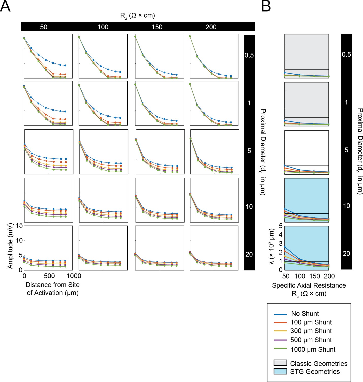
Simulated measurement of electrotonus in neurites in cables with unsealed proximal ends.
Measurement of λeffective was simulated in NEURON as shown in Figure 1A,D and plotted for a representative subspace of the cable model library with a specific membrane resistance (Rm) of 10,000 Ω*cm2, range of specific axial resistances (Ra): 50, 100, 150, and 200 Ω*cm, and a subset of morphologies with proximal diameters (d0) of 0.5, 1, 5, 10, and 20 µm and a constant distal diameter (d1) of 0.5 µm. This cross-section of the cable model library is equivalent to those generating the yellow curves in the leftmost column of plots in Figure 1—figure supplement 1 to Figure 1 (the blue curves in this figure are equivalent to the yellow curves in Figure 1—figure supplement 1 to Figure 1). (A) Array of plots depicting voltage response amplitude (mV) plotted as a function of increasing distance from the site of activation (at 0 µm), illustrating electrotonic decrement of the propagating voltage signal with distance in cables with different Ra values (columns, proximal diameters (d0, rows), and shunt sizes (different colors in key). A large load or unsealed end was achieved by situating a second branch (diameter of 10 µm; Rm and Ra consistent with the parent cable) 300 µm from the proximal end. The size of this shunt was altered by simply changing the length of this appended branch (100, 300, 500, 1000 µm long as in legend). Consistent with Figure 1B and D, while the finer cables yield large distal events that decrement immensely with distance, wider cables yield smaller events that decrement less with distance. It is evident in these plots that unsealed ends with increasing shunt sizes modulate the gain of these curves. (B) Plots showing effective λ as a function of Ra (Ω*cm) for varying shunt sizes (plotted by color as in key). Black horizontal line depicts λeffective = 1 mm, as a reference. Each plot, from top to bottom, corresponds to a different diameter at the proximal end of the cable (d0). The blue shaded region denotes neurite geometries reminiscent of those observed experimentally in secondary neurites of STG neurons (Otopalik et al., 2017a). The gray shaded region indicates neurite geometries that are consistent with those measured in a variety of vertebrate pyramidal neurons. Increasing the shunt size decreases the effective λ across a range of Ra values. However, cables with larger proximal diameters (shaded in blue) and smaller Ra values are somewhat resilient and present λeffective>1 mm for shunts as along as 1 mm.
Figure 2 with 3 supplements
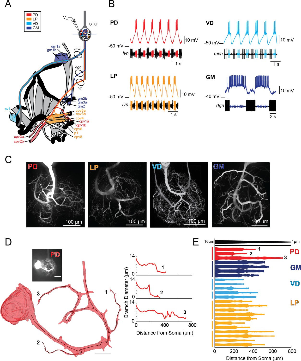
Characteristics of four identified STG neuron types.
(A) Bilateral innervation patterns of each neuron type, depicted on one side of the dissected foregut. Axons from the four neuron types project from the STG (top) and project to specific muscle groups (indicated with the same colors). The axonal spiking activity for each of these neurons can be recorded with extracellularly nerve recordings at the circled locations on the mvn, dgn, and lvn nerves. (B) Each neuron type can be identified electrophysiologically by matching intracellular firing patterns with concurrent extracellular recordings of nerves known to contain their axons (as shown in A). (C) Representative z-projections show complex neurite trees for each neuron type acquired at 40x magnification. (D) Left: volumetric reconstruction of soma and a subset of branches in an example PD neuron (inset scale bar 200 µm and black scale ball in reconstruction is 40 µm). Both the full reconstruction (red – used to measure cross-sectional area and infer branch diameter) and skeleton reconstruction (black line – as used to calculate path distance of glutamate photo-uncaging sites to soma in Figure 3 and Supplements to Figure 3) are shown. Right: the diameter of the three branches shown in reconstruction as a function of distance from the soma. (E) Flattened representations of the reconstructed branches from a subset of preparations. The width of the shape at a given distance from the soma is directly proportional to the inferred diameter of the branch at that distance. Top: Scaled linearly-tapered branch (black) for reference with a starting width of 10 µm (at x = 0 µm) distal width of 1 µm (at x = 800 µm). For branches in D (right) and E, cross-sectional area and path distance were calculated for each node in the skeleton. Inferred diameters were calculated by treating the cross-section as if it were circular; in actuality very few, if any, cross-sections were exact circles. To reduce abrupt irregularities in the inferred diameter, the plots displayed here are a running average with a sliding window of three skeletal nodes. For A- E: PD = Pyloric Dilator; LP = Lateral Pyloric; VD = Ventricular Dilator; GM = Gastric Mill; lvn = lateral ventricular nerve; dgn = dorsal gastric nerve; mvn = medial ventricular nerve. For all subfigures: red = PD, orange = LP; light blue = VD; dark blue = GM.
Figure 2—figure supplement 1
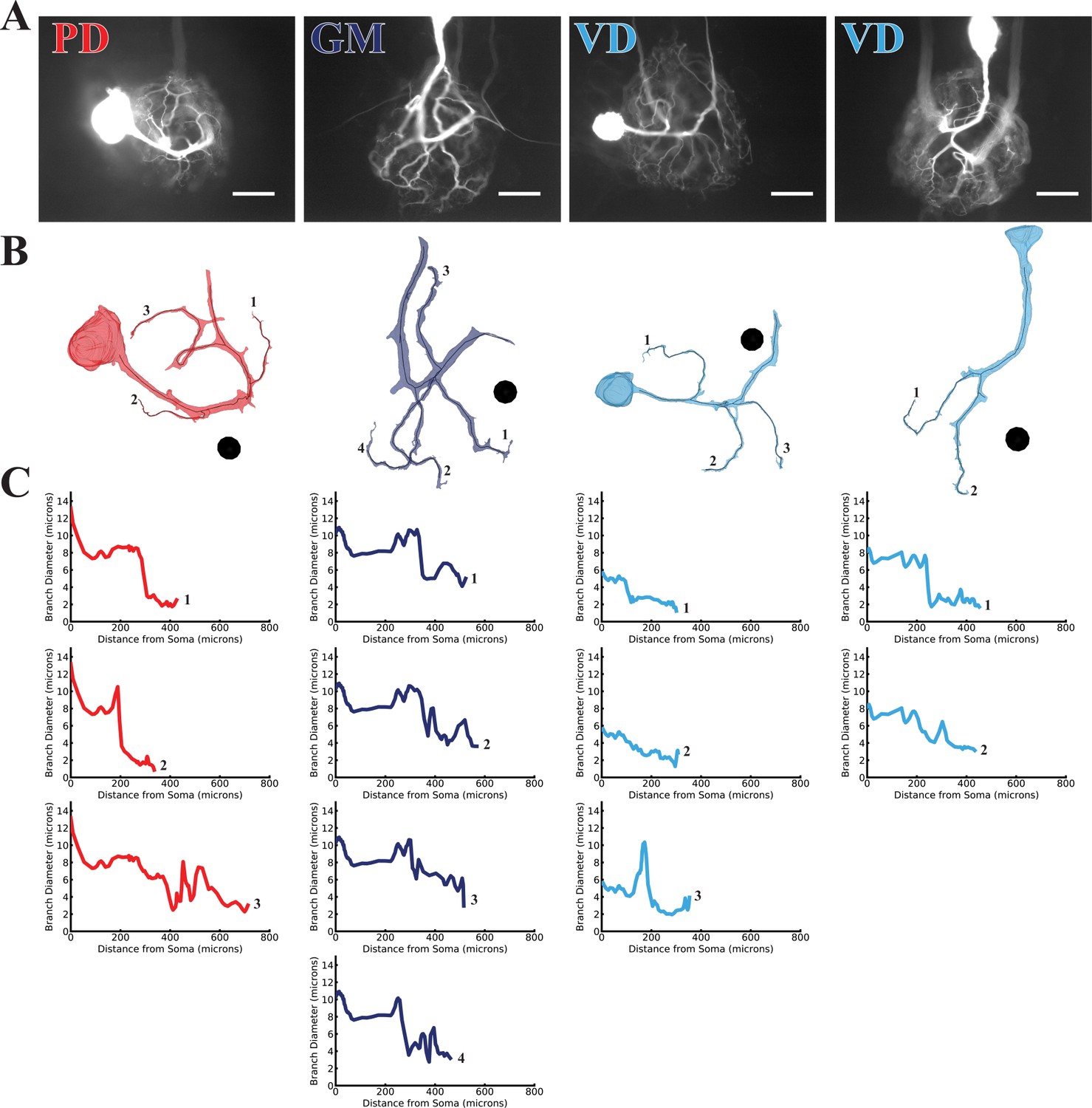
Branch diameter on uncaged branches as a function of path distance from soma.
(A) Low magnification (20x objective) images of four dye-filled neurons used in uncaging experiments. The PD, GM, and both VD preparations were imaged after a post-photo-uncaging dye-fill with Lucifer Yellow (LY). Scale bars 200 µm. (B) Manually-generated 3-D reconstructions and skeletons of the primary neurite and the subset of branches that were uncaged upon. Reconstructions were made from a montage of confocal image stacks. Black balls are objects placed within the 3-D environment for scale; each is 40 µm in diameter. (C) The branch diameter as a function of path distance along each uncaged branch (numerical labels match each plot with the corresponding branch in B). Cross-sectional area and path distance were calculated for each node in the skeleton. Diameters were calculated by treating the cross-sectional area as if it were circular. To reduce irregularities caused by small node-to-node differences in cross-sectional area, the plots show the running average of three nodes’ path distance versus the running average of the diameter inferred from their cross-sectional areas.
Figure 2—figure supplement 2

Branch diameter on uncaged branches as a function of path distance from soma.
(A) Low magnification (20x objective) images of three dye-filled neurons used in uncaging experiments. The three LP preparations were imaged with an Alexa Fluor 488 fills prior to the Lucifer Yellow (LY) fill. Scale bars 200 µm. (B) Manually-generated 3-D reconstructions and skeletons of the primary neurite and the subset of branches that were uncaged upon. Reconstructions were made from a montage of confocal image stacks. Black balls are objects placed within the 3-D environment for scale; each is 40 µm in diameter. (C) The branch diameter as a function of path distance along each uncaged branch (numerical labels match each plot with the corresponding branch in B). Cross-sectional area and path distance were calculated for each node in the skeleton. Diameters were calculated by treating the cross-sectional area as if it were circular. To reduce irregularities caused by small node-to-node differences in cross-sectional area, the plots show the running average of three nodes’ path distance versus the running average of the diameter inferred from their cross-sectional areas.
Figure 2—figure supplement 3

Simulated measurement of electrotonus in neurites with varying degrees of taper.
Measurement of λeffective was simulated in NEURON as shown in Figure 1A,D. (A) seven cable geometries with varying degrees of taper: from a gradual linear taper (blue, top) to abrupt step-reduction (red, bottom). All cables assessed in this simulation exhibit diameters that decrease by 80% from proximal (d0) to distal end (d1). (B) This array of plots shows λeffective as a function of specific axial resistance (Ra in Ω*cm) for cables with different d0 and d1 values (columns), specific membrane resistances (Rm in Ω*cm2), and varying degrees of taper (colors correspond to morphologies shown in Part A). The plots shaded in blue denotes neurite geometries reminiscent of those observed experimentally in STG neurites (Figure 2E; Otopalik et al., 2017a).
Figure 3 with 4 supplements

Variable response amplitudes and invariant apparent reversal potentials (Erevs) across STG neuronal structures.
(A and B) Glutamate photo-uncaging and measurement of apparent Erevs in a representative PD neurite. (A) Fluorescence images of an Alexa Fluor 488 dye-fill showing the neurite tree at 20x magnification and a single branch at 40x magnification (outlined in blue on the 20x image). Glutamate photo-uncaging sites are indicated with colored circles and corresponding responses (measured at the soma) for each site are shown. At each site, inhibitory events were evoked with a 1 ms, 405 nm laser pulse at a starting somatic membrane potential of −50 mV. (B) Plots showing evoked response amplitude (∆V) as a function of somatic membrane potential (Vm). At each site, glutamate responses were evoked at varying somatic membrane potentials (achieved with two-electrode current clamp). These data were fit with a linear regression (colored lines) and the Erev for each site was calculated as the x-intercept of this fit (values for each site shown on bottom right of each plot). C. Response amplitudes plotted as a function of distance from the somatic recording site for each neuron type. Maximum response amplitudes were measured at −50 mV for individual sites and normalized to the maximum response amplitude within each neuron (−1 is equivalent to the maximum response within individual neurons). There was no quantitative relationship between response amplitude and distance (supported by poorly fit linear regression analyses in Table 1). D. Apparent Erevs for each site were normalized to the mean apparent Erevs within each neuron (one is representative to the mean). Horizontal black lines denote boundaries of ±5% of the mean apparent Erevs and serve as a graphical depiction of the low variance in apparent Erevs within each neuron for sites as far as 800–1000 µm away from the soma. Raw response amplitudes and apparent Erevs for individual sites in individual neurons are shown in Figure 3—figure supplement 1–4 to Figure 3.
Figure 3—figure supplement 1

PD response magnitudes and apparent reversal potentials (Erevs) as a function of distance from the somatic recording site.
(A) Maximum response amplitudes were measured at −50 mV for individual sites. Each plot shows response amplitudes for many sites in one neuron. (B) Apparent Erevs measured for each site. Each plot shows apparent Erevs for many sites in one neuron. B and D are the same normalized plots of response amplitude and apparent Erevs, respectively, shown in Figure 3.
Figure 3—figure supplement 2

LP response magnitudes and apparent reversal potentials (Erevs) as a function of distance from the somatic recording site.
(A) Maximum response amplitudes were measured at −50 mV for individual sites. Each plot shows response amplitudes for many sites in one neuron. (B) Apparent Erevs measured for each site. Each plot shows apparent Erevs for many sites in one neuron. B and D are the same normalized plots of response amplitude and apparent Erevs, respectively, shown in Figure 3.
Figure 3—figure supplement 3

VD response magnitudes and apparent reversal potentials (Erevs) as a function of distance from the somatic recording site.
(A) Maximum response amplitudes were measured at −50 mV for individual sites. Each plot shows response amplitudes for many sites in one neuron. (B) Apparent Erevs measured for each site. Each plot shows apparent Erevs for many sites in one neuron. B and D are the same normalized plots of response amplitude and apparent Erevs, respectively, shown in Figure 3.
Figure 3—figure supplement 4

GM response magnitudes and apparent reversal potentials (Erevs) as a function of distance from the somatic recording site.
(A) Maximum response amplitudes were measured at −50 mV for individual sites. Each plot shows response amplitudes for many sites in one neuron. (B) Apparent Erevs measured for each site. Each plot shows apparent Erevs for many sites in one neuron. B and D are the same normalized plots of response amplitude and apparent Erevs, respectively, shown in Figure 3.
Figure 4 with 2 supplements
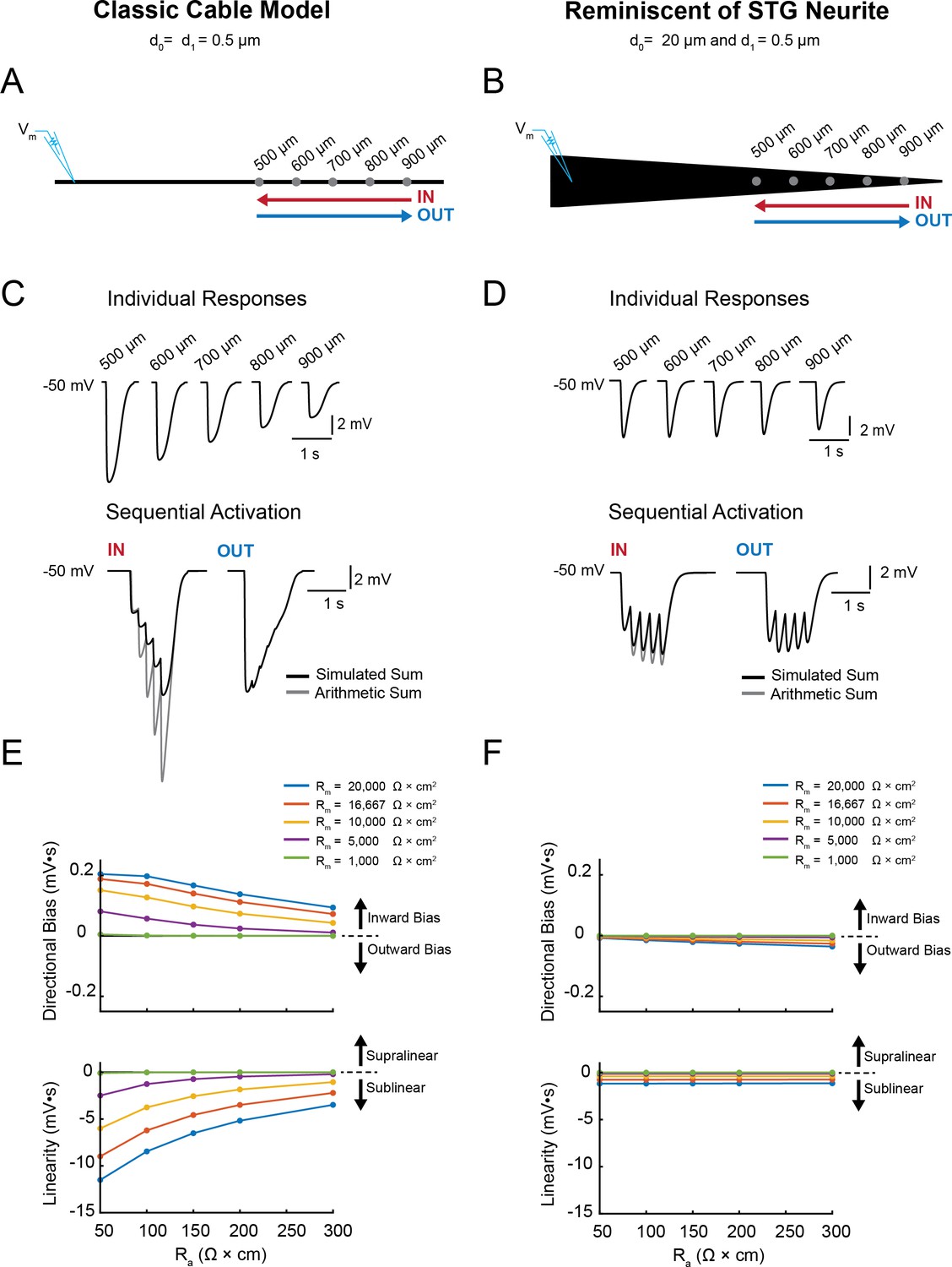
Simulating voltage summation in neurites with diverse passive properties and geometries.
Voltage summation experiments were simulated in NEURON. Inhibitory potentials were evoked at five sites (500, 600, 700, 800, and 900 µm away from the recording electrode) individually or in sequence at 5 Hz in the inward or outward directions relative to the recording site. (A-C) summarizes results from a classic cable model without a tapering geometry, as in Figure 1B. (D-F) summarizes results from a cable model with neurite geometry reminiscent of that observed in STG neurons, as in Figure 1D. (A) Schematic showing a classic cable model simulation for a 0.5 µm, uniform-diameter cable. (B) Simulated traces show consequence of activating individual sites (top) and sequential activation in either direction (below), as depicted by colored arrows in (A). (C) Quantification of directional bias and linearity for 0.5 µm-diameter cables varying in their passive properties. Top: directional bias as a function of specific axial resistivity (Ra in Ω*cm). Directional bias was calculated as inward integral minus the outward integral; positive values suggest an inward bias, whereas negative values suggest an outward bias. Points close to the y = 0 suggest no directional preference. Bottom: Linearity as a function of Ra. Linearity was calculated as the inward integral minus the integral of the arithmetic sum of events evoked at individual sites (as in B, top); positive values suggest supralinear summation, whereas negative values suggest sublinear voltage summation. Points close to the y = 0 suggest linear summation. All plots show data for a range of specific membrane resistivity (Rm in Ω*cm2) values in different colors (indicated in the key below). Data for the full simulation exploring a broad parameter space are shown in Figure 4—figure supplement 1 and 2 to Figure 4. (D) Schematic showing a cable model simulation for a neurite that tapers from 20 µm at the recording end (d0) to 0.5 µm at the distal end (d1). (E) Simulated traces for activation of individual sites (top) and sequential activation in either direction (below), as depicted by colored arrows in D. (F) Directional bias and linearity plotted as a function of Ra and varying Rm values (indicated in key) for a cable with the geometry shown in D. B and E: Rm = 10000 Ω*cm2 and Ra = 100 Ω*cm.
Figure 4—figure supplement 1
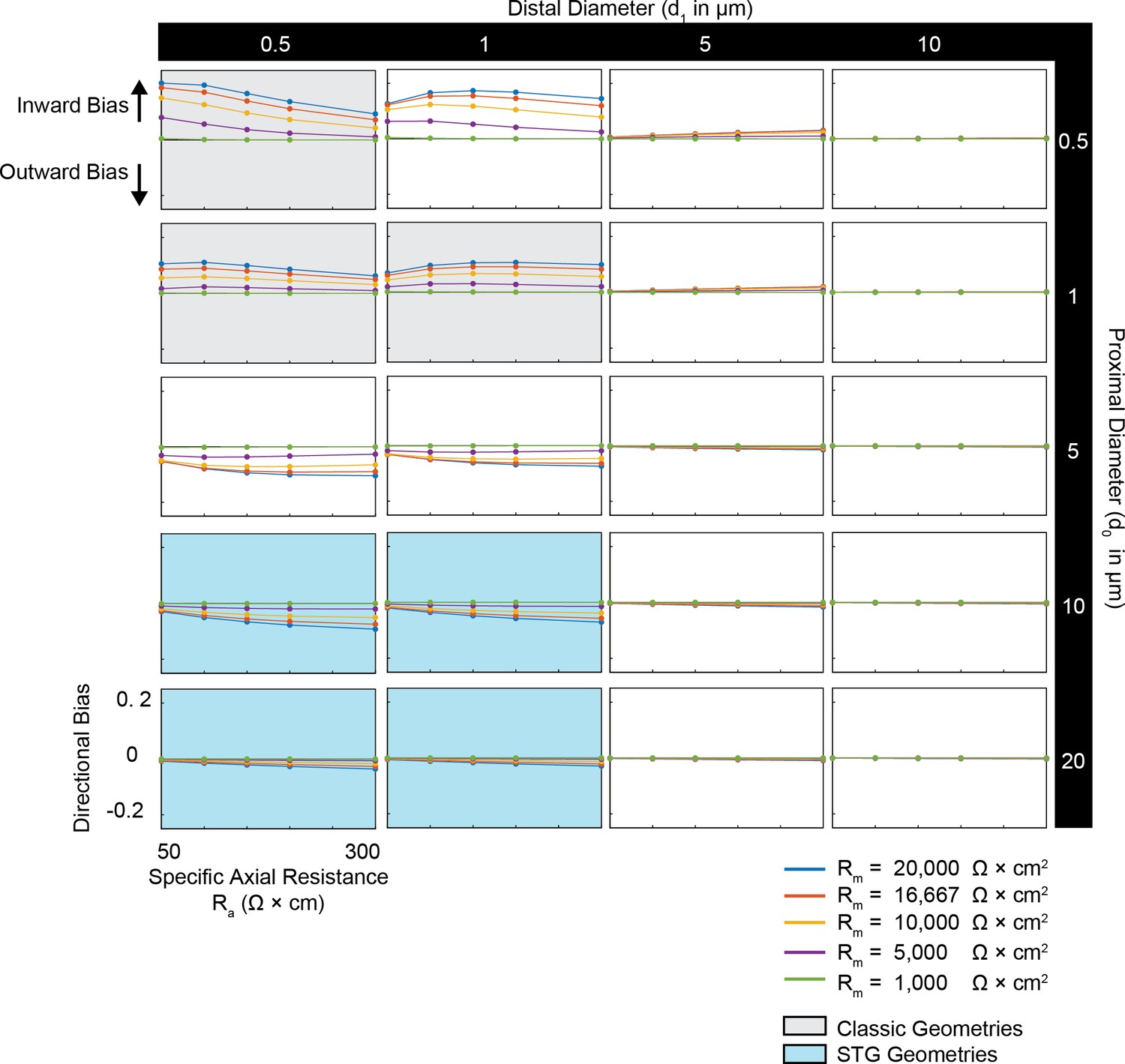
Simulated measurement of directional bias of voltage summation in neurites with diverse passive properties and geometries.
Voltage summation experiments were simulated in NEURON as shown in Figure 4A,B. This array of plots shows directional bias, calculated as the integral of the inward voltage sum minus the outward voltage sum, as a function of specific axial resistance (R<strike>a</strike> in Ω*cm) for a range of different specific membrane resistance (Rm in Ω*cm2) values (by color, shown in key). Positive data points suggest an inward bias, whereas negative values suggest an outward bias. Points close to y = 0 show no directional preference. Each column of plots corresponds to a different diameter at the distal end of the cable (d1), and each row of plots corresponds to a different diameter at the recording end of the cable (d0). These geometries are illustrated in Figure 1A. The blue shaded region denotes neurite geometries with tapers reminiscent of those observed experimentally in secondary neurites of actual STG neurons (Otopalik et al., 2017a). The gray shaded region indicates neurite geometries that are consistent with those measured in a variety of vertebrate pyramidal neurons.
Figure 4—figure supplement 2
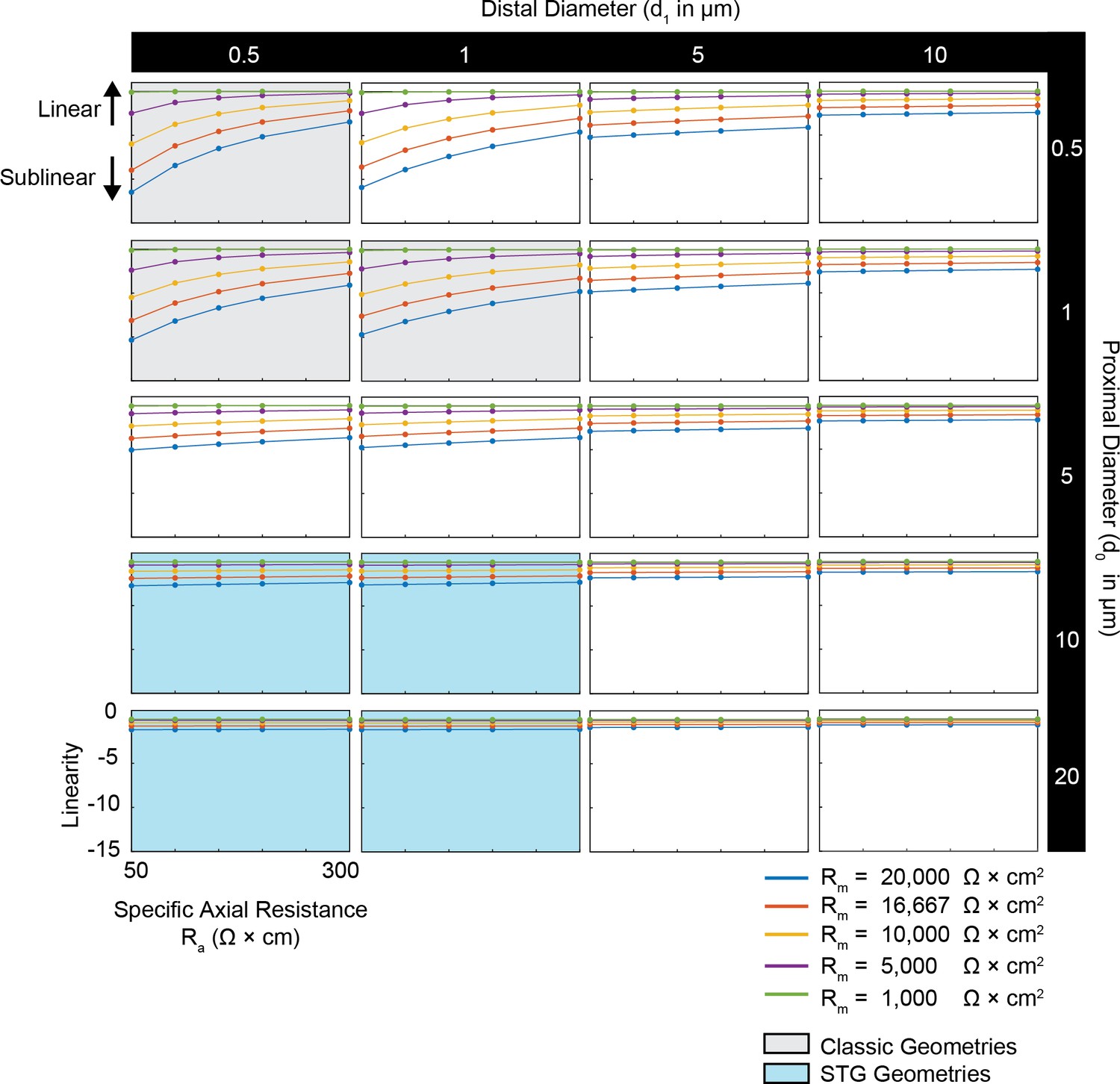
Simulated measurement of voltage summation arithmetic in neurites with diverse passive properties and geometries.
Voltage summation experiments were simulated in NEURON as shown in Figure 4A,B. This array of plots shows the linearity of voltage summation, calculated as the integral of the inward voltage sum minus the arithmetic sum of the individual events, as a function of specific axial resistance (Ra in Ω*cm) for a range of different specific membrane resistance (Rm in Ω*cm2) values (by color, shown in key). Positive data points suggest supralinear summation, whereas negative values suggest sublinear summation. Points close to y = 0 indicate linear summation. Each column of plots corresponds to a different diameter at the distal end of the cable (d1), and each row of plots corresponds to a different diameter at the recording end of the cable (d0). These geometries are illustrated in Figure 1A. The blue shaded region denotes neurite geometries with tapers reminiscent of those observed experimentally in secondary neurites of actual STG neurons (Otopalik et al., 2017a). The gray shaded region indicates neurite geometries that are consistent with those measured in a variety of vertebrate pyramidal neurons.
Figure 5 with 4 supplements
Directional sensitivity of voltage propagation in four STG neuron types.
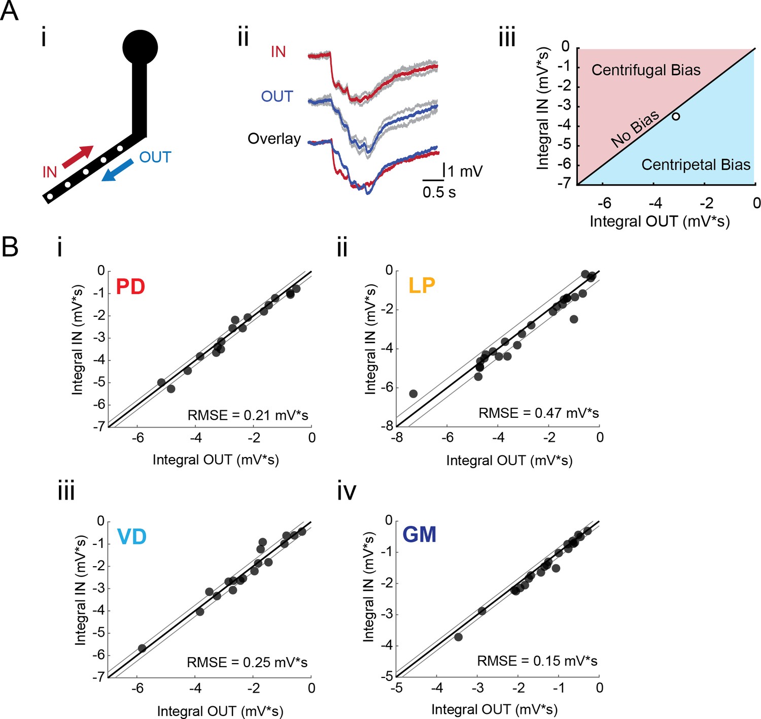
(A) (i) 4–6 sites on single secondary neurites were sequentially photo-activated at 5 Hz in the inward (IN) or outward (OUT) directions. The integrals (ii) of these inhibitory summation responses were calculated as the area above the trace (in mV*s) and plotted against each other as shown in (iii). As plotted, any points that lie to the right of the identity line (shaded in blue) show a centripetal, or inward bias, whereas any points that lie to the left of the identity line (shaded in red) show an outward, or centrifugal, bias. Any points near or on the identity line are unbiased (as is the case with the example traces shown in (ii), depicted with the white data point in (iii)). (B) Directional bias plots for numerous branches within neuron type: (i) 19 branches from 6 PD neurons, (ii) 27 branches from 9 LP neurons, (iii) 20 branches from 5 VD neurons, (iv) 22 branches from five neurons. These data were fit to the identity line, and the root-mean-square error (RMSE) boundaries for this fit is plotted in gray lines.
Figure 5—figure supplement 1
Directional sensitivity and arithmetic of voltage propagation in PD neurons.
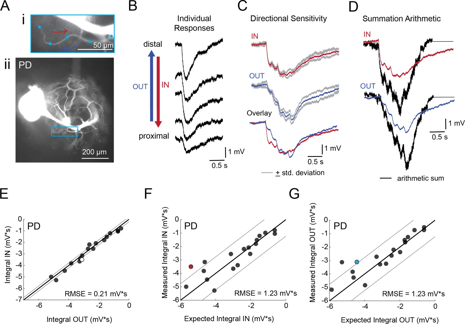
(A) Representative images depicting one secondary neurite branch (i) at 40x magnification and (ii) in context of the entire dye-filled structure at 20x magnification. Arrows indicate inward (IN; red) and outward (OUT; blue) activation. (B) Response evoked at −50 mV for individual sites shown in A from most distal site (top) to most proximal site (bottom). (C) Comparison of mean summed voltage response for inward (red) and outward (blue) activation sequences at 5 Hz for the branch shown in A (mean calculated from three trials; the mean +standard deviation (gray) shows little variation across trials). (D) Comparison of evoked responses (red, blue) to the arithmetic sum of the individual responses (summed with a 200 ms offset in either direction) for the branch in A. In this case, the measured responses are much less than the arithmetic sum expected for linear voltage summation. (E) Plot of the measured inward integral (mV*s) as a function of the measured outward integral (mV*s). Points to the left of the identity line suggest an outward bias, points to the right of the identity line suggest an inward bias. Points near or on the identity suggest no directional preference. The white data point denotes the branch shown in part A. (F-G) Plots of the measured integral (inward or outward, respectively, in mV*s) as a function of the integral expected from arithmetic summation of the responses at individual sites. Points to the left of the identity line suggest sublinear summation, points to the right of the identity line suggest supralinear summation. Points near or on the identity line suggest linear summation. Colored data points denote the data from the branch shown in A. In E-G: Show data for 19 branches from 6 PD neurons; RMSE boundaries are plotted as gray lines and show the goodness of fit to the identity line.
Figure 5—figure supplement 2
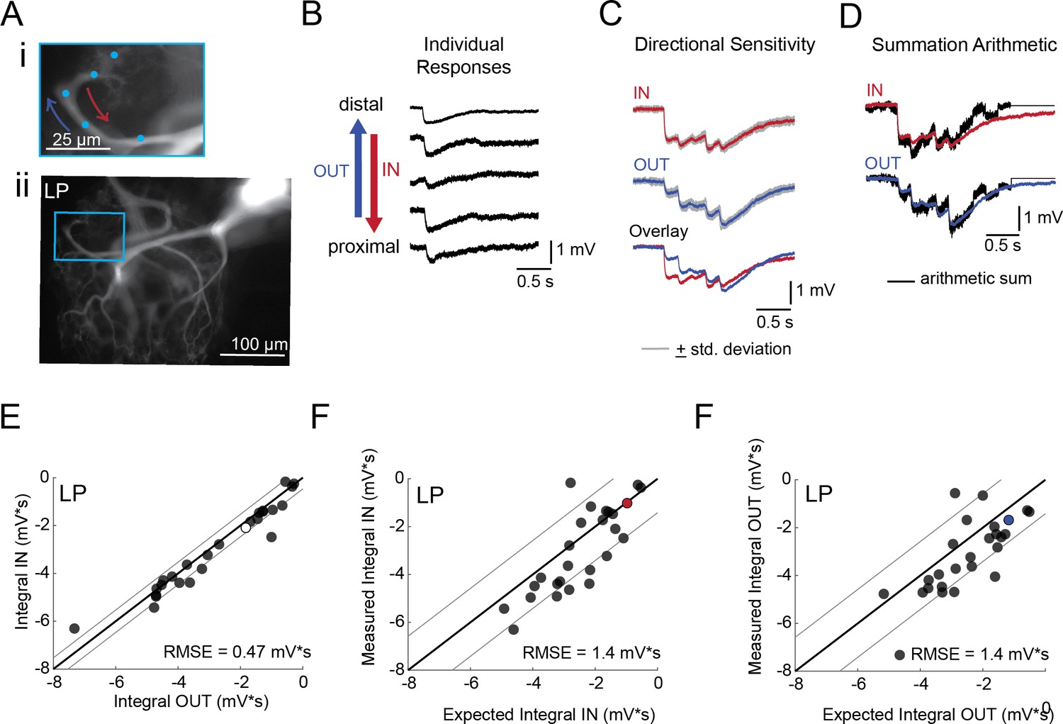
Directional sensitivity and arithmetic of voltage propagation in LP neurons.
(A) Representative images depicting one secondary neurite branch (i) at 40x magnification and (ii) in context of the entire dye-filled structure at 20x magnification. Arrows indicate inward (IN; red) and outward (OUT; blue) activation. (B) Response evoked at −50 mV for individual sites shown in A from most distal site (top) to most proximal site (bottom). (C) Comparison of mean summed voltage response for inward (red) and outward (blue) activation sequences at 5 Hz for the branch shown in A (mean calculated from three trials; the mean +standard deviation (gray) shows little variation across trials). (D) Comparison of evoked responses (red, blue) to the arithmetic sum of the individual responses (summed with a 200 ms offset in either direction) for the branch in A. In this case, the measured responses are similar to the arithmetic sum. (E) Plot of the measured inward integral (mV*s) as a function of the measured outward integral (mV*s). Points to the left of the identity line suggest an outward bias, points to the right of the identity line suggest an inward bias. Points near or on the identity suggest no directional preference. The white data point denotes the branch shown in part A. (F-G) Plots of the measured integral (inward or outward, respectively, in mV*s) as a function of the integral expected from arithmetic summation of the responses at individual sites. Points to the left of the identity line suggest sublinear summation, points to the right of the identity line suggest supralinear summation. Points near or on the identity line suggest linear summation. Colored data points denote the data from the branch shown in A. In E-G: Show data for 26 branches from 9 LP neurons; RMSE boundaries are plotted as gray lines and show the goodness of fit to the identity line.
Figure 5—figure supplement 3
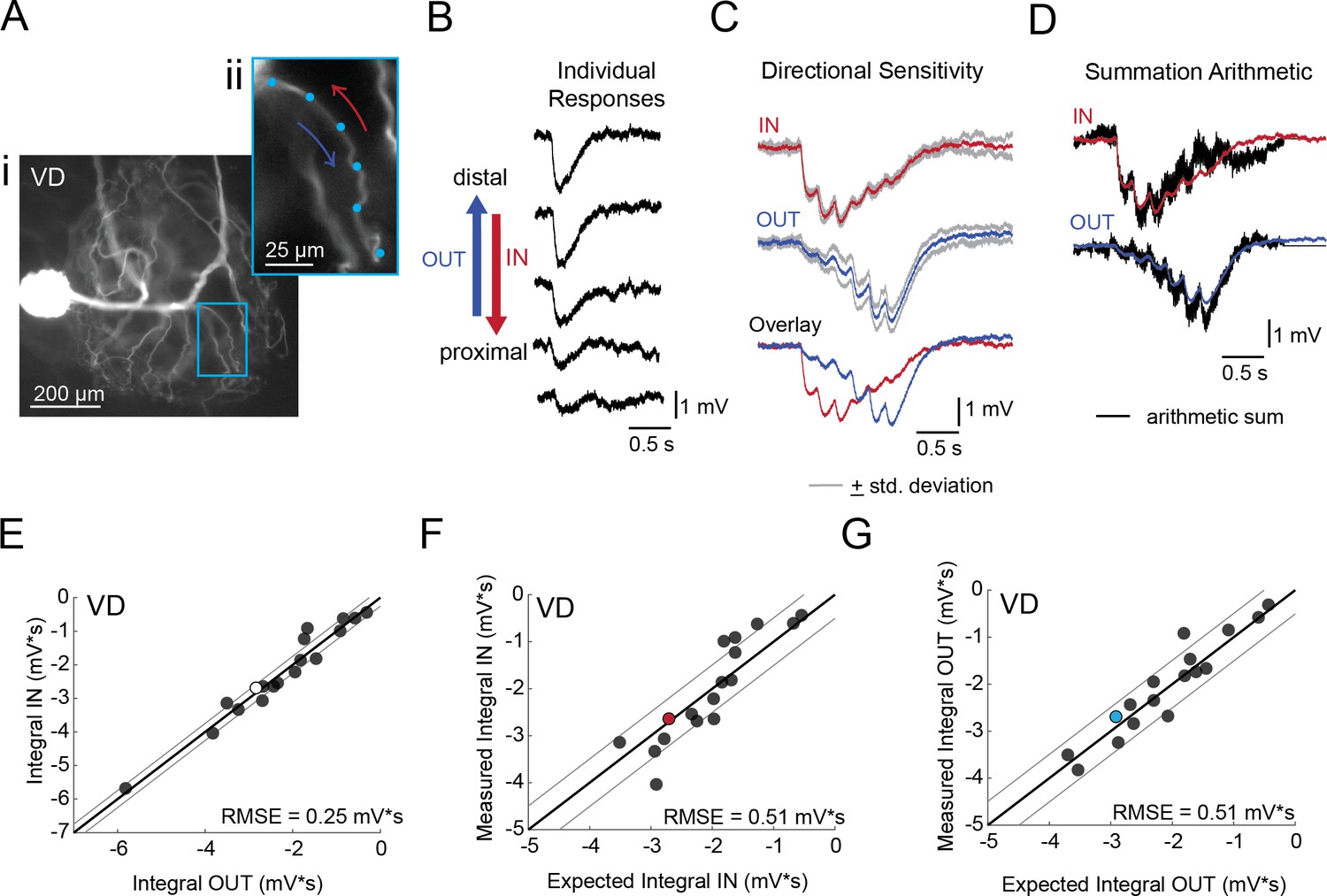
Directional sensitivity and arithmetic of voltage propagation in VD neurons.
(A) Representative images depicting one secondary neurite branch (i) at 40x magnification and (ii) in context of the entire dye-filled structure at 20x magnification. Arrows indicate inward (IN; red) and outward (OUT; blue) activation. (B) Response evoked at −50 mV for individual sites shown in A from most distal site (top) to most proximal site (bottom). (C) Comparison of mean summed voltage response for inward (red) and outward (blue) activation sequences at 5 Hz for the branch shown in A (mean calculated from three trials; the mean +standard deviation (gray) shows little variation across trials). (D) Comparison of evoked responses (red, blue) to the arithmetic sum of the individual responses (summed with a 200 ms offset in either direction) for the branch in A. In this case, the measured responses are similar to the arithmetic sums. (E) Plot of the measured inward integral (mV*s) as a function of the measured outward integral (mV*s). Points to the left of the identity line suggest an outward bias, points to the right of the identity line suggest an inward bias. Points near or on the identity suggest no directional preference. The white data point denotes the branch shown in part A. (F-G) Plots of the measured integral (inward or outward, respectively, in mV*s) as a function of the integral expected from arithmetic summation of the responses at individual sites. Points to the left of the identity line suggest sublinear summation, points to the right of the identity line suggest supralinear summation. Points near or on the identity line suggest linear summation. Colored data points denote the data from the branch shown in A. In (E-G) Show data for 18 branches from 5 VD neurons; RMSE boundaries are plotted as gray lines and show the goodness of fit to the identity line.
Figure 5—figure supplement 4

Directional sensitivity and arithmetic of voltage propagation in GM neurons.
(A) Representative images depicting one secondary neurite branch (i) at 40x magnification and (ii) in context of the entire dye-filled structure at 20x magnification. Arrows indicate inward (IN; red) and outward (OUT; blue) activation. (B) Response evoked at −50 mV for individual sites shown in A from most distal site (top) to most proximal site (bottom). (C) Comparison of mean summed voltage response for inward (red) and outward (blue) activation sequences at 5 Hz for the branch shown in A (mean calculated from three trials; the mean +standard deviation (gray) shows little variation across trials). (D) Comparison of evoked responses (red, blue) to the arithmetic sum of the individual responses (summed with a 200 ms offset in either direction) for the branch in A. In this case, the measured responses are similar to the arithmetic sums. (E) Plot of the measured inward integral (mV*s) as a function of the measured outward integral (mV*s). Points to the left of the identity line suggest an outward bias, points to the right of the identity line suggest an inward bias. Points near or on the identity suggest no directional preference. The white data point denotes the branch shown in part A. (F-G) Plots of the measured integral (inward or outward, respectively, in mV*s) as a function of the integral expected from arithmetic summation of the responses at individual sites. Points to the left of the identity line suggest sublinear summation, points to the right of the identity line suggest supralinear summation. Points near or on the identity line suggest linear summation. Colored data points denote the data from the branch shown in A. In (E-G) Show data for 22 branches from 5 VD neurons; RMSE boundaries are plotted as gray lines and show the goodness of fit to the identity line.
Figure 6
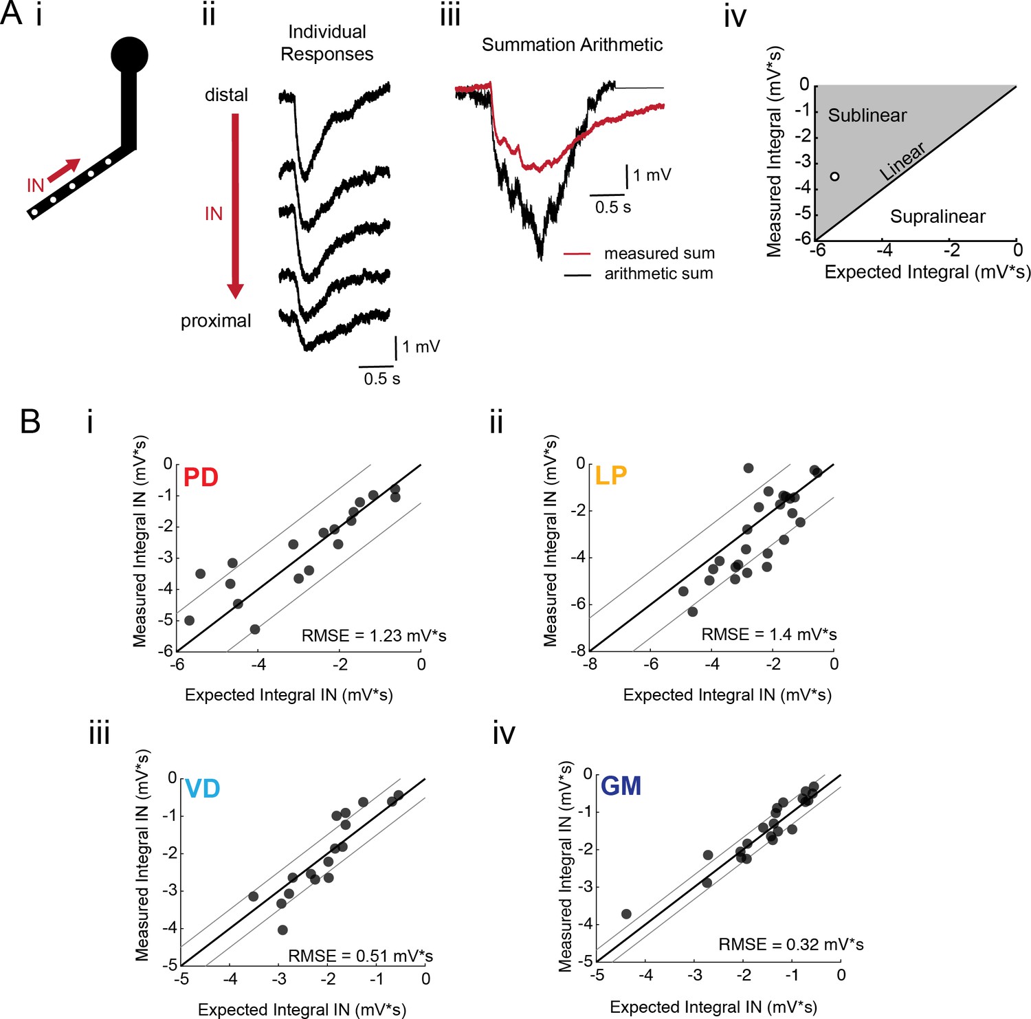
Arithmetic of voltage propagation in four neuron types.
(A) (i) 4–6 sites spaced 50–100 µm apart on the same secondary neurite were sequentially photo-activated at 5 Hz in the inward (IN) direction. (ii) Raw responses at individual sites from most distal (top) to most proximal (bottom) for one representative PD branch. (iii) Comparison of the inward voltage sum to the arithmetic sum for photo-activation of the individual sites (the traces shown in (ii) were summed with a 200 ms offset). (iv) The integrals (mV*s) of the measured responses were plotted against that of the expected arithmetic sum. This provides a graphical depiction of the linearity of voltage summation for each branch. Points to the left of the identity line suggest sublinear summation, points to the right of the identity line suggest supralinear summation, and points near or on the identity line suggest linear summation. The singular point depicted in (iv) depicts voltage summation for the responses shown in (iii). In this case, the measured voltage had a lesser integral than the arithmetic sum and therefore showed sublinear summation. (B) (i–iv) Plots showing the measured integrals as a function of the expected integral for the arithmetic sum for the inward activation of many branches within the four neuron types: (i) 19 branches from 6 PD neurons, (ii) 27 branches from 9 LP neurons, (iii) 20 branches from 5 VD neurons, (iv) 22 branches from five neurons. These real data were fit to the identity line, and the root-mean-square error (RMSE) boundaries for this fit is plotted in gray lines.
Tables
Table 1
Linear regression analyses for response amplitudes and apparent reversal potentials (Erevs) as a function of distance from the somatic recording site for sites in individual neurons or pooled by cell type.
The data contributing to these analyses are shown graphically in Figure 3C and D and Figure 3—figure supplement 1–4 to Figure 3.
| Amplitude vs. Distance | Apparent Erev vs. Distance | ||||||||
|---|---|---|---|---|---|---|---|---|---|
| Neuron | Sites | MSE | R | p | Slope (mV/µm | MSE | R | p | Slope (mV/µm) |
| PD | 30 | 0.08 | 0.05 | 7.98E-01 | 1.67E-04 | 13.61 | 0.17 | 4.22E-01 | -7.23E-03 |
| PD | 23 | 0.15 | -0.05 | 8.38E-01 | -1.03E-04 | 4.66 | -0.73 | 8.43E-05 | -1.35E-02 |
| PD | 10 | 0.05 | -0.06 | 8.28E-01 | -1.77E-04 | 6.65 | -0.42 | 2.26E-01 | -1.60E-02 |
| PD | 23 | 0.37 | -0.47 | 2.05E-02 | -1.56E-03 | 15.13 | -0.19 | 3.88E-01 | -3.87E-03 |
| PD | 20 | 0.40 | -0.18 | 4.26E-01 | -6.35E-04 | 17.96 | 0.05 | 8.50E-01 | 1.05E-03 |
| PD | 23 | 0.77 | 0.40 | 5.18E-02 | 2.62E-03 | 32.09 | 0.37 | 8.55E-02 | 1.62E-02 |
| PDMEAN | 21.5 | 0.30 | -0.05 | 4.94E-01 | 5.18E-05 | 11.60 | -0.29 | 3.77E-01 | -7.91E-03 |
| PDSD | 6.5 | 0.27 | 0.29 | 3.86E-01 | 1.40E-03 | 9.79 | 0.38 | 3.04E-01 | 1.16E-02 |
| LP | 11 | 0.14 | 0.43 | 1.23E-01 | 5.87E-04 | 12.09 | -0.81 | 2.67E-03 | -1.54E-02 |
| LP | 26 | 0.50 | -0.02 | 9.25E-01 | -1.15E-04 | 5.07 | -0.19 | 3.08E-01 | -4.00E-03 |
| LP | 25 | 0.17 | -0.15 | 4.75E-01 | -5.56E-04 | 14.18 | -0.17 | 4.16E-01 | -5.79E-03 |
| LP | 25 | 0.34 | -0.40 | 4.70E-02 | -1.56E-03 | 5.75 | -0.09 | 6.75E-01 | -2.15E-03 |
| LP | 24 | 0.51 | 0.02 | 9.30E-01 | 7.01E-05 | 0.70 | 0.55 | 5.00E-03 | 7.26E-03 |
| LPMEAN | 22.2 | 0.33 | -0.02 | 5.00E-01 | -3.15E-04 | 10.16 | -0.14 | 2.81E-01 | -4.02E-03 |
| LPSD | 6.3 | 0.18 | 0.30 | 4.22E-01 | 8.08E-04 | 5.45 | 0.48 | 2.86E-01 | 8.12E-03 |
| VD | 27 | 0.31 | 0.05 | 7.95E-01 | 2.32E-04 | 193.71 | -0.35 | 7.64E-02 | -4.17E-02 |
| VD | 19 | 0.54 | -0.53 | 3.49E-03 | -6.51E-03 | 28.63 | -0.45 | 5.57E-02 | -3.85E-02 |
| VD | 24 | 0.28 | -0.14 | 5.06E-01 | -2.46E-04 | 41.44 | 0.22 | 3.16E-01 | 5.07E-03 |
| VD | 15 | 0.07 | -0.20 | 3.36E-01 | -3.28E-04 | 15.74 | -0.29 | 2.97E-01 | -7.76E-03 |
| VD | 15 | 0.87 | 0.35 | 4.73E-02 | 1.81E-03 | 33.58 | -0.69 | 3.29E-03 | -5.59E-02 |
| VDMEAN | 20.0 | 0.42 | -0.09 | 3.38E-01 | -1.01E-03 | 62.62 | -0.31 | 1.50E-01 | -2.78E-02 |
| VDSD | 5.4 | 0.31 | 0.33 | 3.29E-01 | 3.19E-03 | 73.87 | 0.33 | 1.46E-01 | 2.54E-02 |
| GM | 10 | 0.04 | -0.84 | 6.83E-04 | -3.23E-03 | 0.56 | -0.14 | 6.93E-01 | -1.17E-03 |
| GM | 28 | 0.09 | -0.53 | 2.02E-03 | -8.74E-04 | 2.09 | 0.31 | 1.13E-01 | 2.49E-03 |
| GM | 25 | 0.64 | -0.24 | 1.78E-01 | -1.12E-03 | 5.56 | -0.13 | 5.28E-01 | -2.23E-03 |
| GM | 20 | 0.09 | -0.41 | 3.50E-02 | -5.76E-04 | 11.76 | 0.17 | 4.76E-01 | 9.37E-03 |
| GM | 19 | 0.03 | -0.57 | 4.56E-03 | -1.14E-03 | 4.03 | -0.24 | 3.26E-01 | -6.53E-03 |
| GMMEAN | 20.4 | 0.18 | -0.52 | 4.41E-02 | -1.39E-03 | 4.80 | -0.01 | 4.27E-01 | 3.85E-04 |
| GMSD | 6.9 | 0.26 | 0.22 | 7.62E-02 | 1.06E-03 | 4.33 | 0.23 | 2.19E-01 | 5.97E-03 |
Table 2
Apparent Mean Erevs, standard deviations (SD) and coefficients of variance (CV) for individual neurons and within neuron type.
https://doi.org/10.7554/eLife.41728.015| Neuron | Sites | Branches | Mean Erev (mV) | SD (mV) | CV |
|---|---|---|---|---|---|
| PD | 30 | 6 | -64.70 | 3.80 | 0.06 |
| PD | 23 | 4 | -66.30 | 3.20 | 0.05 |
| PD | 10 | 3 | -74.30 | 3.00 | 0.04 |
| PD | 23 | 4 | -64.18 | 4.05 | 0.06 |
| PD | 20 | 4 | -69.56 | 4.35 | 0.06 |
| PD | 23 | 4 | -83.00 | 6.22 | 0.08 |
| PDMEAN | 21.5 | 4.2 | -70.34 | 4.10 | 0.06 |
| LP | 11 | 2 | -65.72 | 6.18 | 0.09 |
| LP | 26 | 5 | -72.82 | 2.33 | 0.03 |
| LP | 25 | 5 | -71.87 | 3.89 | 0.05 |
| LP | 25 | 5 | -81.67 | 4.07 | 0.05 |
| LP | 24 | 5 | -71.87 | 3.89 | 0.05 |
| LPMEAN | 22.2 | 4.4 | -72.79 | 4.07 | 0.05 |
| VD | 27 | 4 | -76.22 | 3.75 | 0.05 |
| VD | 19 | 4 | -80.83 | 6.14 | 0.08 |
| VD | 24 | 4 | -83.86 | 6.75 | 0.08 |
| VD | 15 | 4 | -74.81 | 4.29 | 0.06 |
| VD | 15 | 5 | -77.84 | 8.23 | 0.11 |
| VDMEAN | 20 | 4.2 | -78.71 | 5.83 | 0.08 |
| GM | 10 | 2 | -62.33 | 0.80 | 0.01 |
| GM | 28 | 5 | -74.00 | 1.55 | 0.02 |
| GM | 25 | 6 | -74.78 | 2.43 | 0.03 |
| GM | 20 | 5 | -75.42 | 3.57 | 0.05 |
| GM | 19 | 4 | -65.66 | 7.05 | 0.11 |
| GMMEAN | 20.4 | 4.4 | -70.44 | 3.08 | 0.04 |
Additional files
-
Transparent reporting form
- https://doi.org/10.7554/eLife.41728.025
Download links
A two-part list of links to download the article, or parts of the article, in various formats.
Downloads (link to download the article as PDF)
Open citations (links to open the citations from this article in various online reference manager services)
Cite this article (links to download the citations from this article in formats compatible with various reference manager tools)
Neuronal morphologies built for reliable physiology in a rhythmic motor circuit
eLife 8:e41728.
https://doi.org/10.7554/eLife.41728


