Neuronal variability and tuning are balanced to optimize naturalistic self-motion coding in primate vestibular pathways
- McGill University, Canada
- The Johns Hopkins University, United States
Figures
Figure 1 with 1 supplement
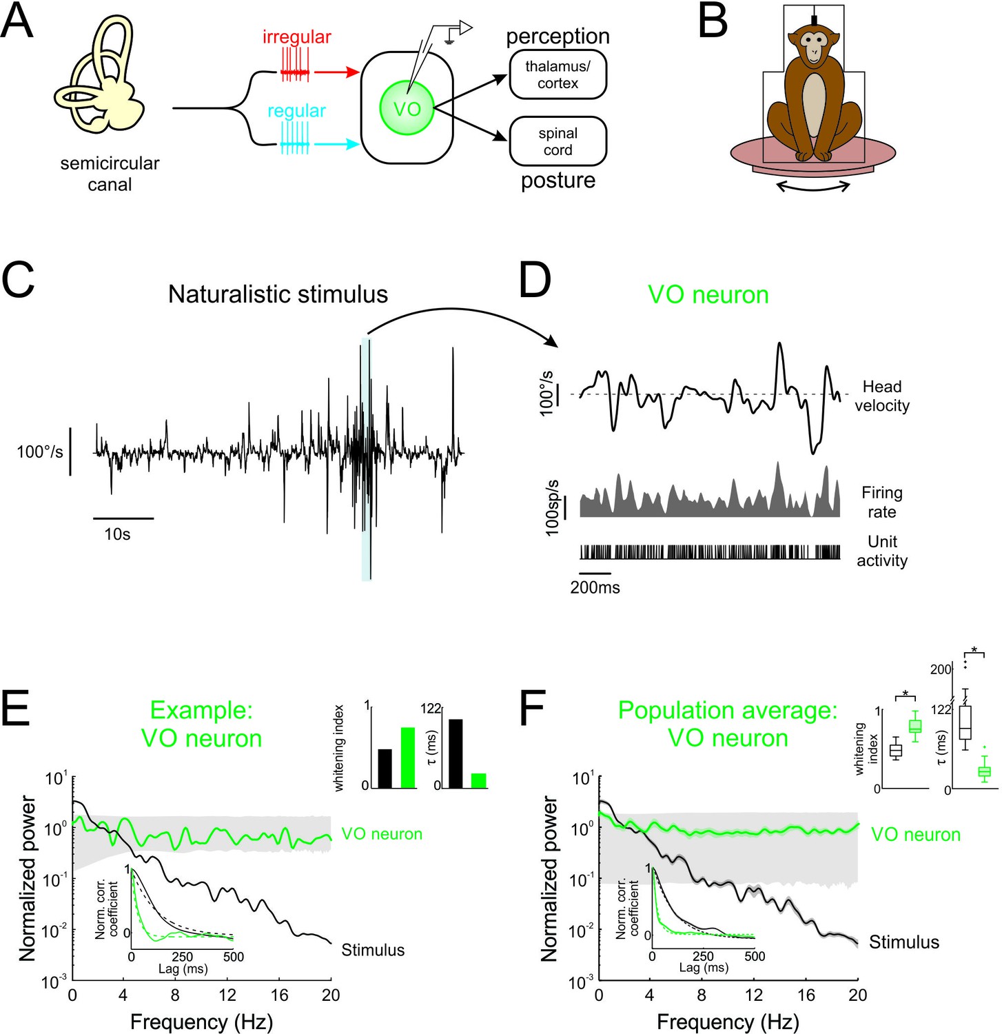
Central vestibular neurons optimally encode natural self-motion stimuli through whitening.
(A) Vestibular afferents provide input to VO neurons in the vestibular nuclei, which in turn project to the spinal cord and higher order brain areas (i.e. thalamus/cortex). Recordings were made from VO neurons. (B) During experiments, the monkey was head-fixed and comfortably seated in a chair placed on a turntable. (C) Naturalistic head velocity during stimulation. (D) Response of an example VO neuron to the head velocity stimulus shown in C. (E) Normalized power spectra of natural stimuli and neural responses for an example VO neuron. Lower left insets shows autocorrelation functions (solid lines) and exponential fits (dashed lines) used to calculate correlation times (lower left), as well as correlation times and whitening indices (upper right). (F) Normalized power spectra of natural stimuli and population averages for VO neurons. Insets show autocorrelation functions (lower left), as well as correlation times and whitening indices (upper right). Whitening indices from VO neurons were significantly higher than those computed from the stimulus (Student’s t-test, p < 0.001, t(26) = 10.9), while their correlation times were significantly lower (Student’s t-test, p < 0.001, t(26) = 16.7). Gray bands show 95% confidence interval obtained using Poisson processes with the same firing rate as the experimental data for which the power spectrum is independent of frequency by definition (see Materials and methods). Error bars show ±1 SEM.
Figure 1—figure supplement 1
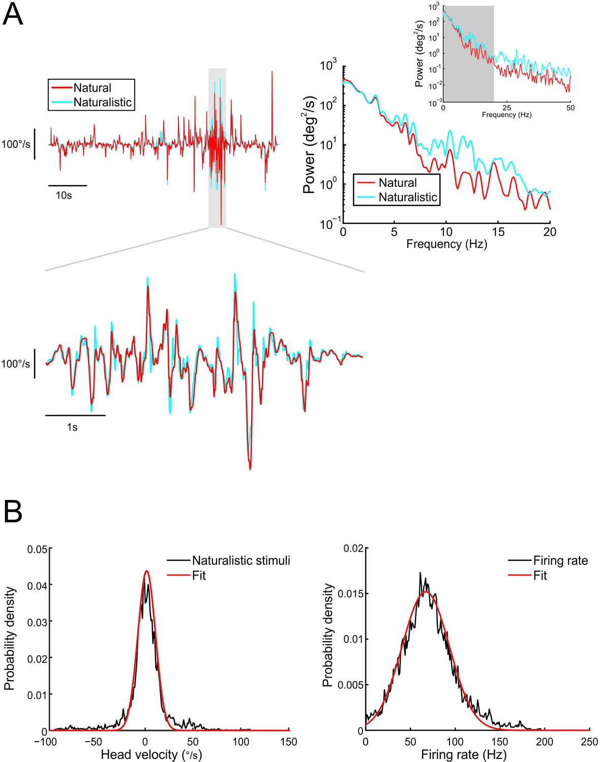
The self-motion stimuli used to elicit responses from vestibular neurons in our study closely matched head movement recordings from freely moving monkeys performing natural behaviors.
(A) Upper left: Head velocity recorded during stimulation (naturalistic: blue trace) and in freely moving animals performing natural everyday activities (natural: red trace). The lower left panel shows both traces during a period of high activity. Upper right: Power spectra of naturalistic (blue) and natural (red) self-motion stimuli. Inset shows power spectra up to 50 Hz. (B) Probability density functions of naturalistic stimuli (left) and firing rate during naturalistic stimuli (right) are well fit by Gaussian distributions.
Figure 2
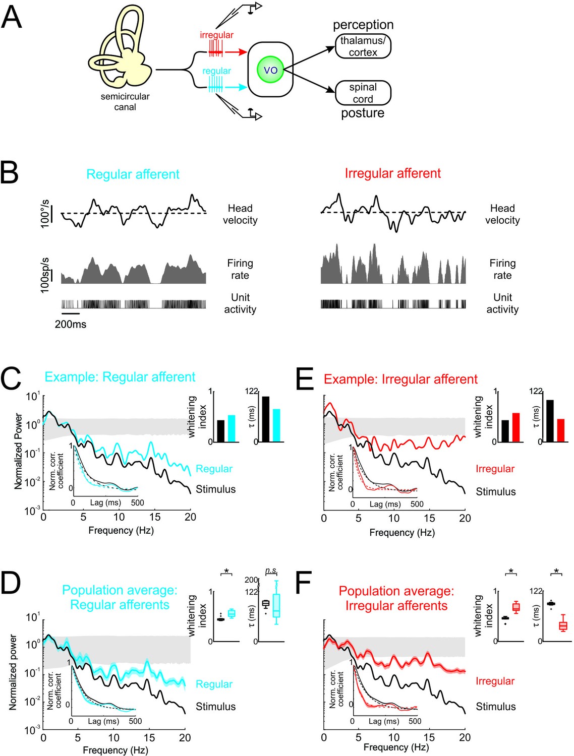
Vestibular afferents do not perform whitening of natural self-motion.
(A) Same diagram as in Figure 1A, except that recordings were made from afferents. (B) Response of example regular (left) and irregular (right) afferents during natural stimulation. (C) Normalized power spectra of natural stimuli (black) and neural response (blue) for the example regular afferent. The lower left inset shows the autocorrelation function of the response (blue) and of the stimulus (black). Solid lines represent autocorrelation functions, while the dashed lines are exponentials fits. The upper right inset shows the whitening index (left) and correlation time (right). (D) Normalized population-averaged power spectrum for regular afferents (blue) with that of the stimulus (black). The lower left inset shows the population-averaged response autocorrelation function (blue). The upper right inset shows the population-averaged whitening index (left) and correlation time (right) values. The whitening index was not significantly different than that of the stimulus (Student’s t-test, p = 0.79, t(13)=0.27). The correlation time was significantly lower than that of the stimulus (Student’s t-test, p < 0.001, t(13)=2.9). (E) Normalized power spectra of natural stimuli (black) and neural response (red) for the example irregular afferent. The lower left inset shows the autocorrelation function of the response (red) and of the stimulus (black). Solid lines represent autocorrelation functions, while the dashed lines are exponentials fits. The upper right inset shows the whitening index (left) and correlations time (right). (F) Normalized population-averaged power spectrum for irregular afferents (red) with that of the stimulus (black). The lower left inset shows the population-averaged response autocorrelation function (red). The upper right inset shows the population-averaged whitening index (left) and correlation time (right) values. The whitening index was significantly higher than that of the stimulus (Student’s t-test, p < 0.001, t(11)=2.25). The correlation time was significantly lower than that of the stimulus (Student’s t-test, p < 0.001, t(11)=9.64). Gray bands show 95% confidence interval obtained using Poisson processes with the same firing rate as the experimental data for which the power spectrum is independent of frequency by definition (see Materials and methods). Error bars show ±1 SEM.
Figure 3
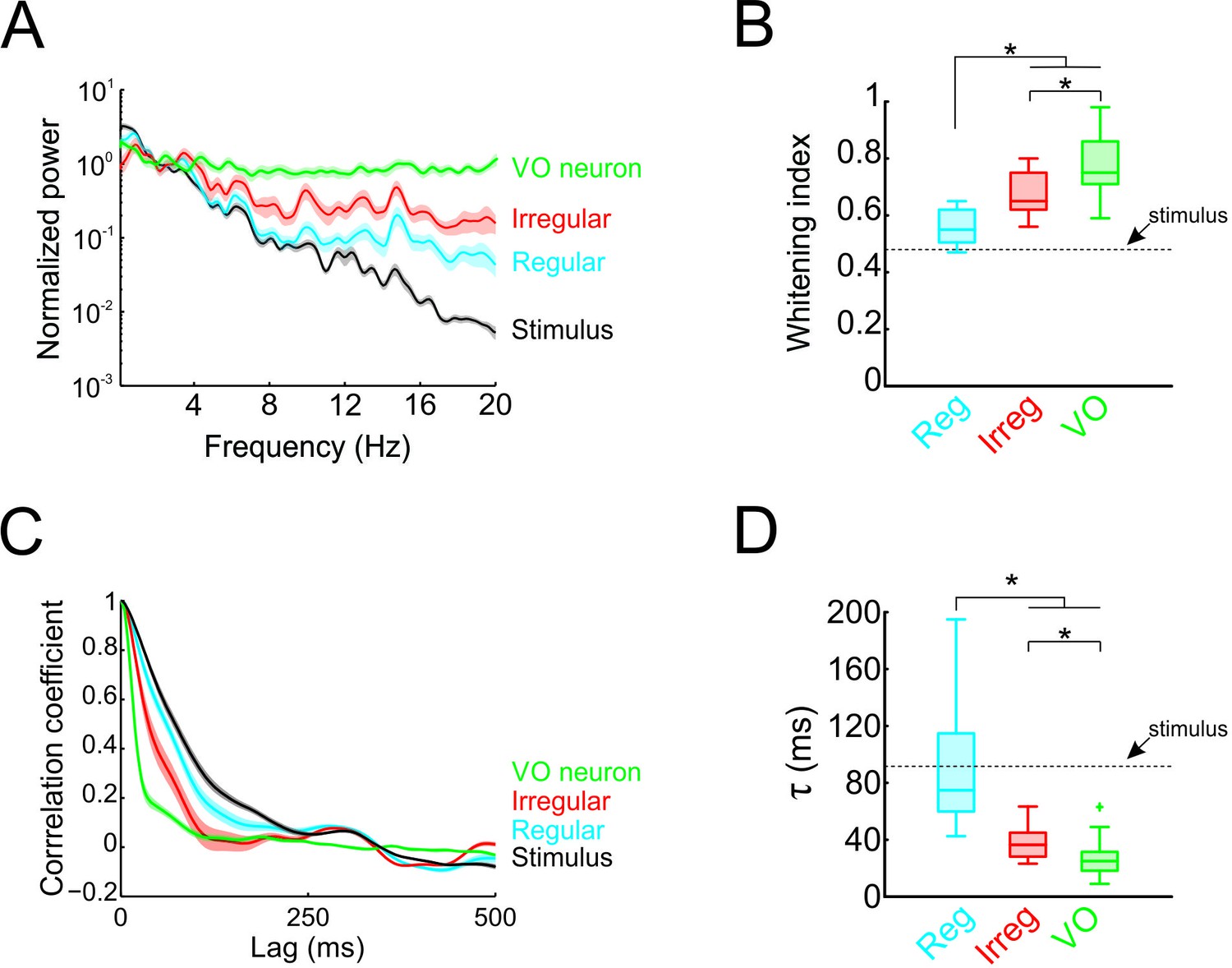
Temporal whitening of neuronal responses occurs sequentially throughout early vestibular pathways.
(A) Normalized power spectra of natural stimuli (black), and neuronal responses of regular (blue), irregular afferents (red), and VO neurons (green). (B) Population-averaged whitening index values for regular afferents (blue, left), irregular afferents (red, middle), and VO neurons (green, right). Values for VO neurons were significantly higher than those of either regular or irregular afferents, while those of irregular afferents were significantly higher than those of regular afferents (one-way ANOVA, p < 0.001, F(2,50)=24.26). (C) Normalized autocorrelation functions of natural stimuli (black), and neuronal responses of regular (blue), irregular afferents (red), and VO neurons (green). (D) Population-averaged correlation time values for regular afferents (blue, left), irregular afferents (red, middle), and VO neurons (green, right). Values for VO neurons were significantly lower than those of either regular or irregular afferents, while those of irregular afferents were significantly lower than those of regular afferents (one-way ANOVA, p < 0.001, F(2,50)=26.68).
Figure 4 with 4 supplements
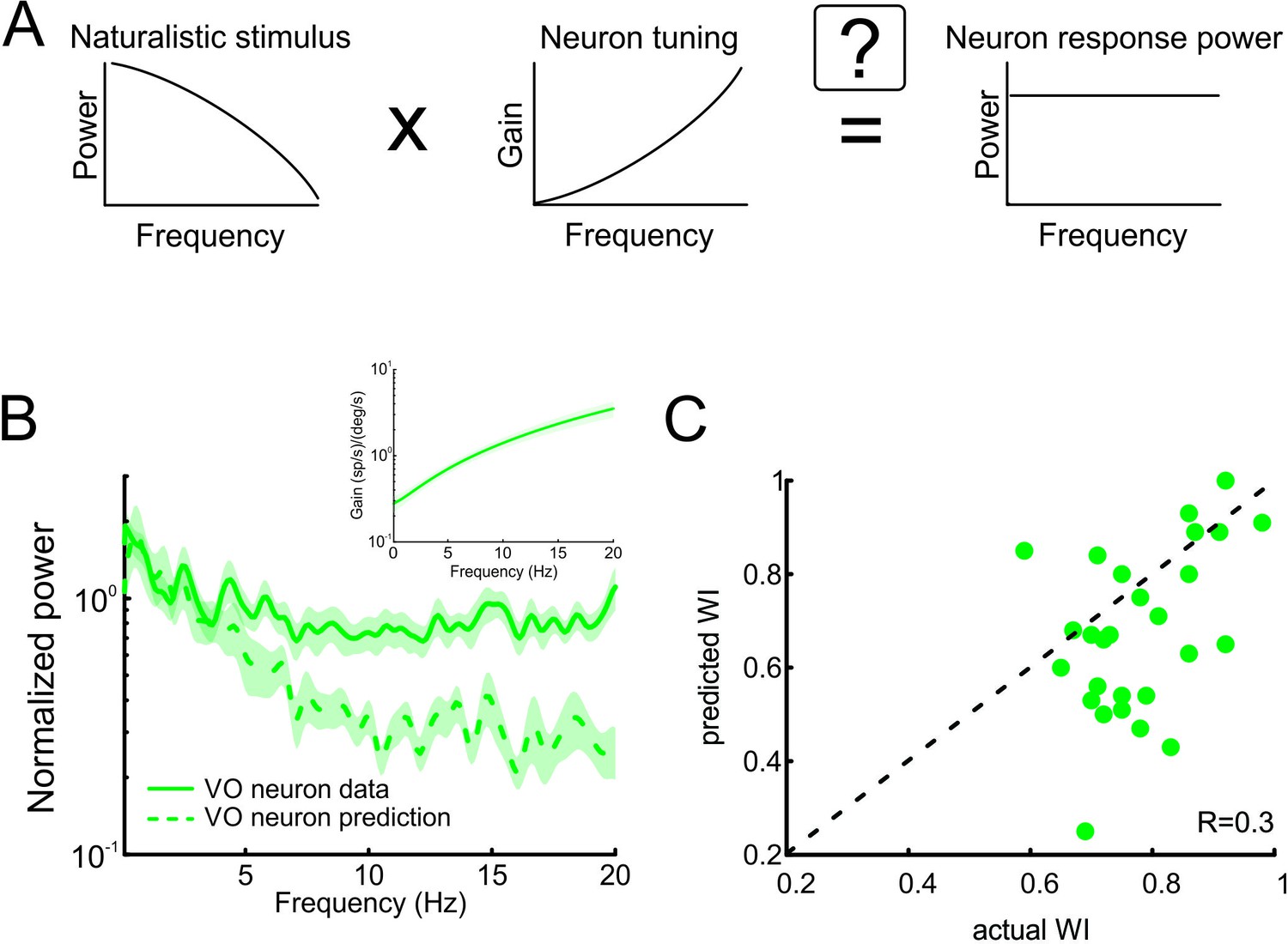
Neural tuning to naturalistic stimulation does not account for the temporally whitened responses of central vestibular neurons to natural stimuli.
(A) Schematic showing how the response to a natural stimulus (right) is assumed to be determined from the stimulus spectrum (left) and the neural tuning function (middle). (B) Normalized population-averaged actual (solid green) and predicted (dashed green) response power spectra for central vestibular neurons. Inset: Population-averaged tuning curve showing gain as a function of frequency for central vestibular neurons. (C) Predicted versus actual whitening indices for central vestibular neurons. Most data points were below the identity line (dashed black).
Figure 4—figure supplement 1

Adding a static nonlinearity does not account for responses of central vestibular neurons to natural stimuli.
Left: Normalized power spectra of neural response (solid green), linear (dashed light green), and nonlinear predictions (dashed dark green). Right: Predicted whitening index values from the nonlinear model were lower than actual values.
Figure 4—figure supplement 2
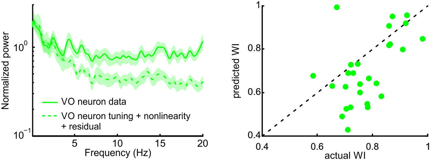
The residual between the actual firing rate and the nonlinear prediction does not account for responses of central vestibular neurons to natural stimuli.
Left: Normalized power spectra of neural responses (solid green) and nonlinear prediction to which the residual power spectrum was added (dashed dark green). Right: Predicted whitening index values were lower than actual values.
Figure 4—figure supplement 3
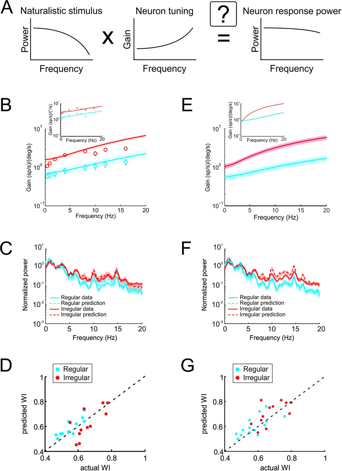
Neural tuning to artificial sinusoidal stimulation and to natural stimulation accounts for responses of afferents to natural stimuli.
(A) Schematic showing how the response to a natural stimulus (right) is assumed to be determined from the stimulus spectrum (left) and the neural tuning function (middle). (B) Population-averaged tuning curves to sinusoidal stimulation for regular (blue) and irregular (red) afferents with best fits (solid lines). The bands show ±1 SEM. Inset: Tuning curves from example regular (blue) and irregular (red) afferents (data points) with best fits (solid lines). (C) Normalized actual response power spectra for regular (blue) and irregular (red) afferents (solid lines) and predictions from tuning to sinusoidal stimulation (dashed lines). (D) Predicted whitening index values versus actual ones for regular (blue) and irregular (red) afferents. (E) Population-averaged tuning curves to naturalistic stimulation for regular (blue) and irregular (red) afferents with best fits (solid lines). The bands show ±1 SEM. Inset: Tuning curves from example regular (blue) and irregular (red) afferents (data points) with best fits (solid lines). (F) Normalized actual response power spectra for regular (blue) and irregular (red) afferents (solid lines) and predictions from tuning to naturalistic stimulation (dashed lines). (G) Predicted whitening index values versus actual ones for regular (blue) and irregular (red) afferents.
Figure 4—figure supplement 4
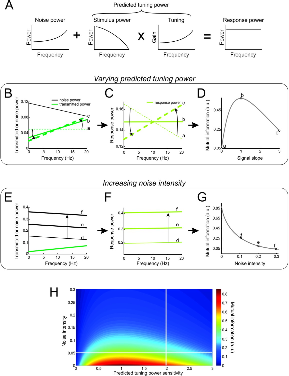
Mutual information is determined from both the noise and transmitted power spectra.
(A) Schematic of our model in which the response power is equal to the sum of the noise power and of the predicted response power (i.e. that obtained by multiplying the stimulus power by the tuning function). (B) Noise power spectrum (black) and three different transmitted power spectra that increase at different rates but with the same area under the curve (green curves). (C) Response power spectra computed from the spectra shown in B. (D) Mutual information as a function of the rate at which the transmitted power spectrum increases. Data points represent the mutual information obtained for the three examples shown in B and C. (E) Noise power spectra and transmitted power spectrum for three different noise intensities. (F) Response power spectra computed for the spectra shown in E. (G) Mutual information as a function of noise intensity. Data points represent mutual information values for examples shown in E and F. (H) Color plot showing mutual information as a function of rate and noise intensity. The horizontal white line shows the scenario considered in B-D, while the vertical white line shows the scenario considered in E-G.
Figure 5
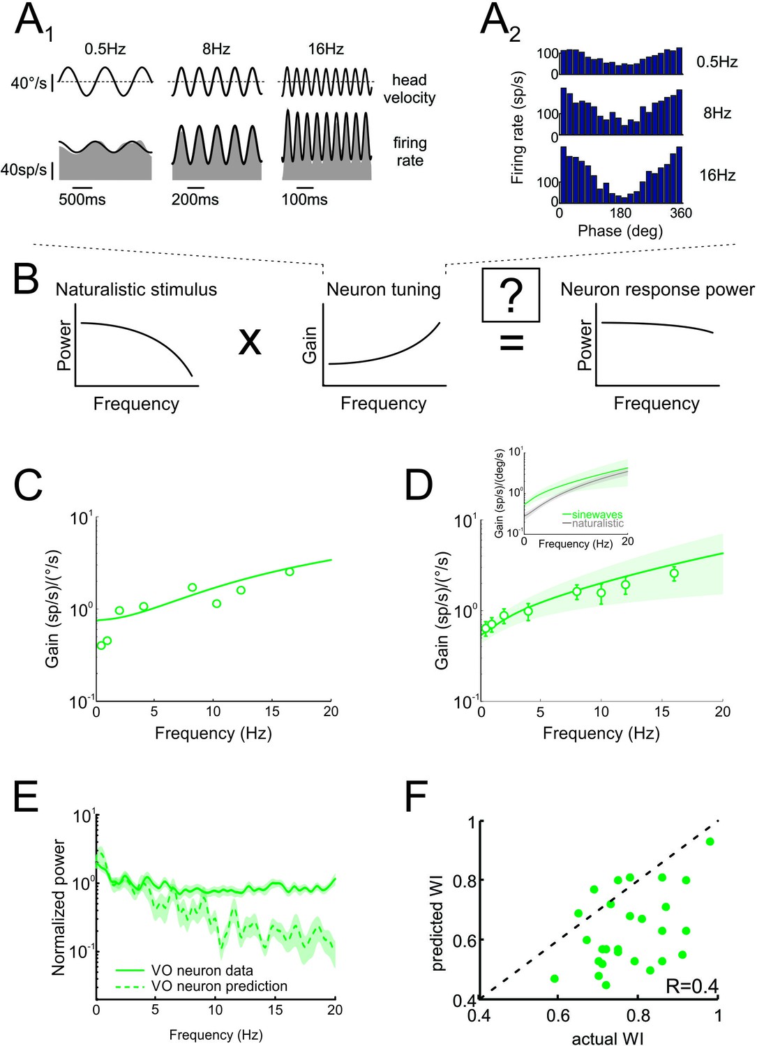
Neural tuning to artificial sinusoidal stimulation does not account for responses of central vestibular neurons to natural stimuli.
(A1) Response of example central vestibular neuron to sinusoidal yaw rotations with frequencies 0.5, 8 and 16 Hz. (A2) Post-stimulus time histogram (PSTH) of this example central vestibular neuron to sinusoidal yaw rotations with frequencies 0.5, 8 and 16 Hz. (B) Schematic showing how the response to a natural stimulus (right) is assumed to be determined from the stimulus spectrum (left) and the neural tuning function (middle). (C) Gain as a function of frequency for an example central vestibular neuron with best fit (solid line). (D) Population-averaged gain as a function of frequency. The solid line is the best fit with bands showing ±1 SEM. (E) Normalized power spectra of neural responses (solid green) and predictions (dashed green) for central vestibular neurons. Inset: Population-averaged tuning curves obtained using naturalistic (gray) and sinusoidal (green) stimulation. Note that the tuning obtained using naturalistic stimulation was lower than that obtained using sinusoidal stimulation at low frequencies, consistent with the fact that central vestibular neurons display a boosting nonlinearity (Massot et al., 2012). (F) Predicted versus actual whitening indices.
Figure 6 with 2 supplements
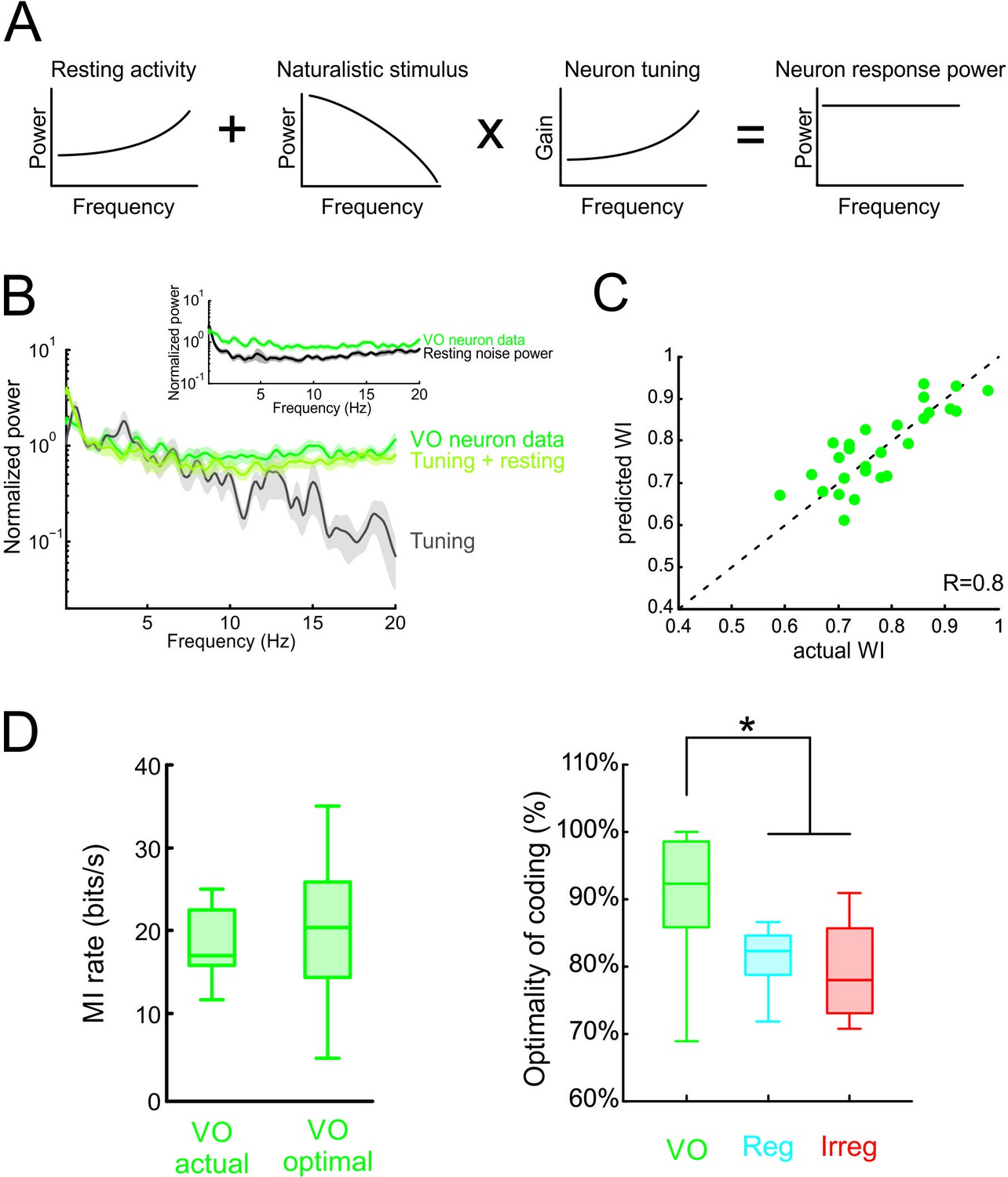
Neural variability and tuning determine whitening of natural self-motion stimuli by central vestibular neurons.
(A) Schematic showing how the response power spectrum (right) can be predicted from the resting activity power spectrum (left) as well as the stimulus power spectrum (middle left) and the neural tuning function (middle right). Specifically, the resting activity power spectrum should compensate the transmitted power spectrum (i.e. that obtained by multiplying the stimulus power by the tuning function) such that the response power spectrum (i.e., the sum of the two) is constant as a function of frequency. (B) Population-averaged actual response power spectrum (dark green) together with the prediction from the resting discharge and tuning (light green). The transmitted power spectrum (grey) is also shown. The inset shows the population-averaged resting discharge (black) and actual response (dark green) power spectra. (C) Predicted versus actual whitening index values for central vestibular neurons. Data points were scattered across the identity line. (D) Left: Population-averaged actual (left) and maximum (right) information rate values for central vestibular neurons. Right: The population-averaged mutual information normalized by the optimal value for VO neurons (green) was significantly greater than that of regular (blue) and irregular (red) afferents (one-way ANOVA, p < 0.001, F(2,50)=14.79). Error bars represent ±1 SEM.
Figure 6—figure supplement 1

Predicting response power spectra of central vestibular neurons using trial-to-trial variability.
(A) Population-averaged resting discharge (gray) and trial-to-trial variability (i.e., the ‘residual’; blue). (B) Population-averaged power spectra of the neural response (green) together with those predicted from tuning alone (black), tuning with resting discharge (dashed green), tuning with trial-to-trial variability (dashed light green). Also shown are the trial-averaged response power spectrum (red) and response power predicted from the trial-averaged response and trial-to-trial variability (dashed red). (C) Predicted vs. actual white index values computed using resting discharge and tuning (green), trial-to-trial variability and tuning (gray), and using trial-to-trial variability and trial-averaged response (red). Bands represent ±1 SEM.
Figure 6—figure supplement 2
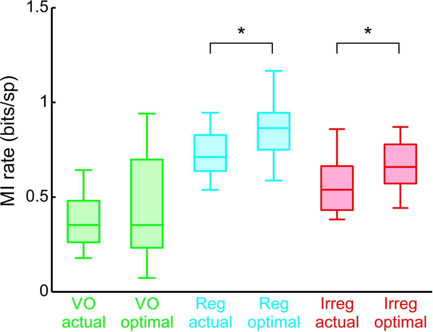
Actual and maximum population-averaged mutual information rate values for central vestibular neurons (green) as well as regular (blue) and irregular (red) afferents.
‘*” indicates statistical significance at the p = 0.05 level using a Student’s t-test (VO neurons: p = 0.2, regular afferents: p = 0.001; irregular afferents: p = 0.008).
Additional files
-
Transparent reporting form
- https://doi.org/10.7554/eLife.43019.015
Download links
A two-part list of links to download the article, or parts of the article, in various formats.
Downloads (link to download the article as PDF)
Open citations (links to open the citations from this article in various online reference manager services)
Cite this article (links to download the citations from this article in formats compatible with various reference manager tools)
Neuronal variability and tuning are balanced to optimize naturalistic self-motion coding in primate vestibular pathways
eLife 7:e43019.
https://doi.org/10.7554/eLife.43019


