Front-end Weber-Fechner gain control enhances the fidelity of combinatorial odor coding
- Yale University, United States
Figures
Figure 1
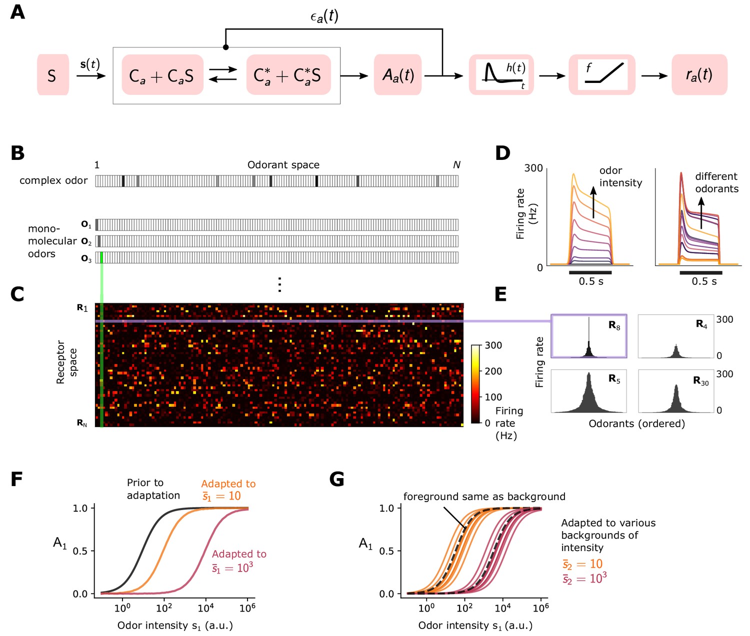
Simple ORN model (Gorur-Shandilya et al., 2017).
(A) Or/Orco complexes of type switch between active and inactive conformations . Binding an exitatory odorant (S in the diagram) favors the active state. The active fraction is determined by the free energy difference between inactive and active conformations of the Or/Orco complex in its unbound state, (in units of ), and by odorant binding with affinity constants and for the active and inactive conformations, respectively (Equations 1-2). Adaptation is mediated by a negative feedback (Nagel and Wilson, 2011) from the activity of the channel onto the free energy difference with timescale . ORN firing rates are generated by passing through a linear temporal filter and a nonlinear thresholding function . (B) Odors are represented by -dimensional vectors , whose components are the concentrations of the individual molecular constituents of . (C) Step-stimulus firing rate of 50 ORNs to the =150 possible monomolecular odorants , given power-law distributed afffinity constants (Si et al., 2019). (D) Temporal responses of a representative ORNs to a pulse stimulus, for a single odorant at several intensities (left), or to many odorants of the same intensity (right). (E) Representative ORN tuning curves (a single row of the response matrix in C, ordered by magnitude). Tuning curves are diverse, mimicking measured responses (Hallem and Carlson, 2006). (F) Dose-response of an ORN before (black) and after adaptation to either a low (yellow) or high (magenta) odor concentration. (G) Same, but the ORN was allowed to first adapt to one of various backgrounds of differing identities, before the foreground (same as in F) was presented. Also shown is the specific case when the foreground and background have the same identity (dashed lines).
Figure 2 with 2 supplements

Front-end adaptation maintains representations of odor identity across background and intensity confounds.
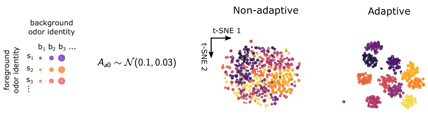
(A) Example t-SNE projection of the 50-dimensional vector of ORN firing rates to two dimensions. Each point represents the firing response to a distinct odor. Nearby points exhibit similarities in corresponding firing rates. (B) t-SNE projection of ORN firing rates, where each point represents the response to foreground odor (point color) on top of a background odor (point size). In the adaptive system, are set to their steady state values given the background odor alone according to Equation 5 with . We assumed for all (we obtain similar results when are randomly distributed; Figure 3—figure supplement 1). Clustering by color implies that responses cluster by foreground odor identity. Since global distances are not preserved by t-SNE, distances between plots cannot be meaningfully compared, and so we do not label the axes with units. Mutual information, in bits, is indicated below the plots. (C) Similar to (B), but now for odors whose concentrations span four decades (represented by point size). Here, the background odor identity is the same for all concentrations. (D) Performance of odor coding as a function of , the magnitude of the deviation from Weber-Fechner’s law (: Weber-Fechner’s scaling; : no adaptation; see Equation 5). Performance is quantified by the mutual information between foreground odor and ORN responses in bits (Materials and methods). Line: same scaling for all ORNs. Dashed: is uniformly distributed between 0 and (i.e. has mean ). (E) Distribution of ORN responses and t-SNE projections for in (D).
Figure 2—figure supplement 1
t-SNE projections when background adapted activity level depends on ORN.
t-SNE projections for non-adaptive () and adaptive () systems, when background firing rates depend on ORN identity. Background active fractions are chosen normally with mean 0.1 and deviation 0.03, corresponding to background firing rates around of 20–40 Hz. .
Figure 2—figure supplement 2

Front-end adaptive feedback preserves information capacity of the ORN sensing repertoire.
Front-end adaptive feedback preserves information capacity of the ORN sensing repertoire. (A) Mutual information between signal and response is calculated at various points in time for an odor environment consisting of two step odors, A and B. Odor A, with concentration , turns on at time and a odor B, with concentration , turns on at some later time . Both odors have similar intensities and similar molecular complexity (). (B) Mutual information as a function of for the non-adaptive system, respectively, at different time points after , corresponding to the dots in (A). The mutual information carried by distinct ORNs is represented by the shaded region; their average is plotted by the heavy line. In the non-adaptive system, the mutual information peaks in the regime of high sensitivity after the arrival of odor A (purple, blue), and shifts leftward with the onset of odor B (teal, green). The leftward shifts occurs since stronger signals are more prone to response saturation (compromising information transfer) as odor B arrives. (C) Same as B, now for the adaptive system. The MI mimics the non-adaptive case at the onset of odor A, before adaptation has kicked in (purple). As the system adapts and responses decrease toward baseline, previously saturating signal intensities now cross the regime of maximal sensitivity, which therefore shifts rightward to higher (dark blue). Much later, but before the arrival of odor B, the ORNs that responded now fire at a similar adapted firing rate ∼30 Hz, irrespective of odor identity, so the mutual information drops to zero. However, having now adjusted its sensitivity to the presence of odor A, the system can respond appropriately to odor B: the MI at is nearly six bits across decades of concentration immediately following (green).
Figure 3 with 6 supplements
Front-end adaptation promotes accurate odor decoding in static and naturalistic odor environments.
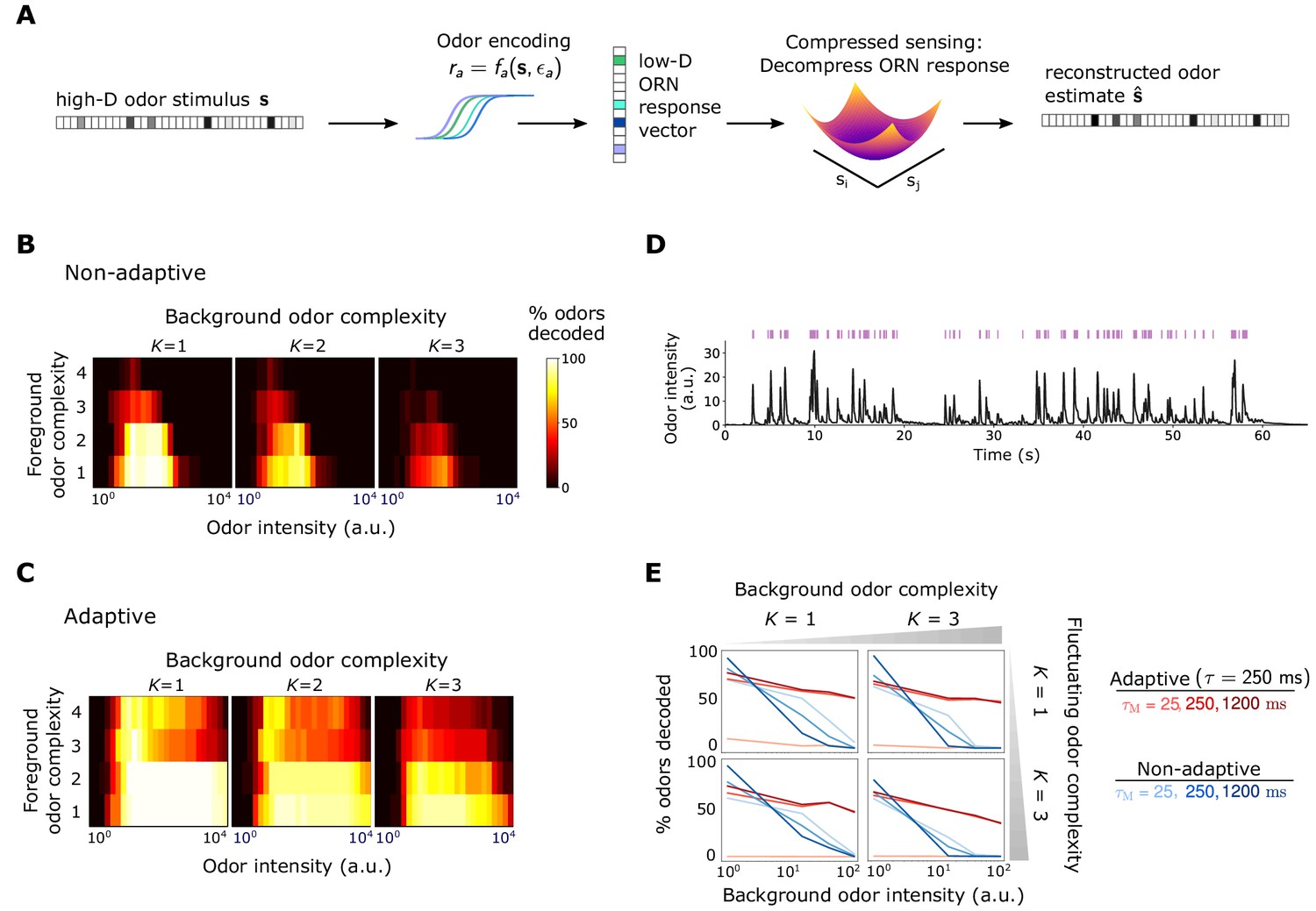
(A) Odor stimuli produce ORN responses via odor-binding and activation and firing machinery, as described by Equations 2-4. Odors are then decoded using compressed sensing optimization. Odors are assumed sparse, with nonzero components, . (B) Decoding accuracy of foreground odors in the presence of background odors, for a system without Weber Law adaptation. (C) Same as (B), with Weber Law adaptation. (D) Recorded trace of naturalistic odor signal; whiffs (signal > 4 a.u.) demarcated by purple bars. This signal is added to static backgrounds of different intensities and complexities. (E) Individual plots show the percent of accurately decoded odor whiffs as a function of background odor intensity, for the non-adaptive (blue) and adaptive (red) systems, for different (line shades).
Figure 3—figure supplement 1
Decoding accuracy for system with ORN-dependent adaptive timescales .
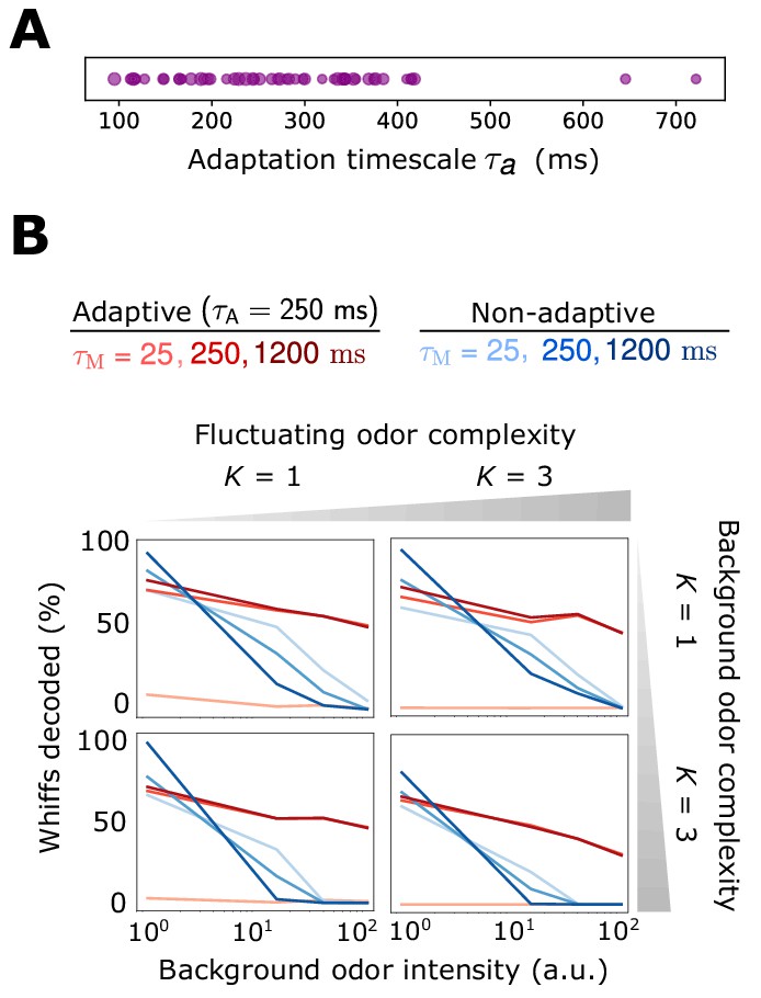
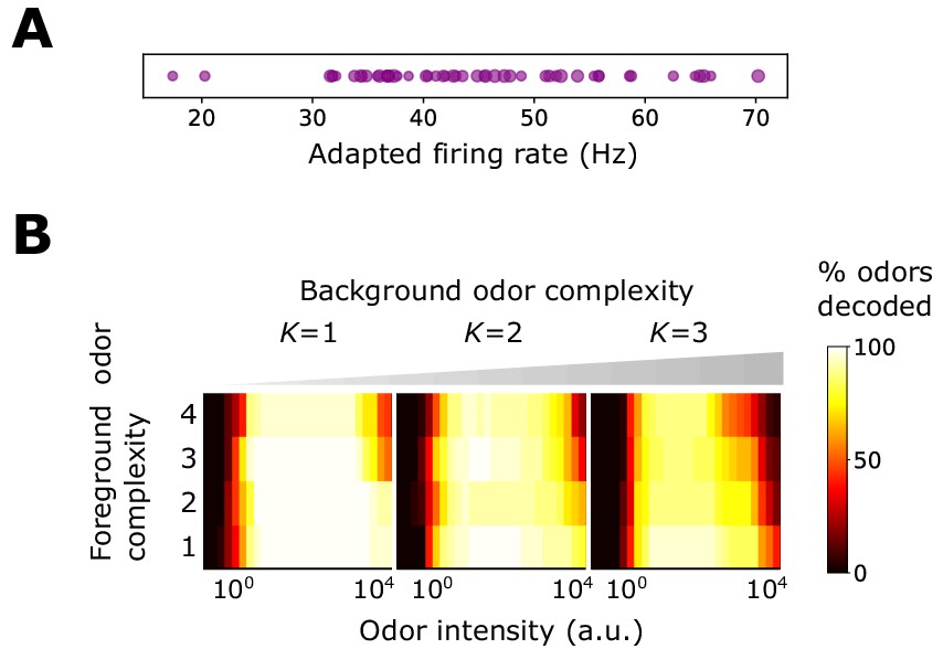
Decoding accuracy for system with ORN-dependent adaptive timescales . (A) Distribution of timescales for all ORNs (purple dots). Here, where as in the main text and . (B) Individual plots show the percent of accurately decoded odor whiffs (same fluctuating odor signal used in the main text) as a function of background odor intensity, for the non-adaptive (blue) and adaptive (red) systems, for different (line shades). Plots are arrayed by the complexity of the naturalistic signal (column-wise) and the complexity of the background odor (row-wise). .
Figure 3—figure supplement 2
Decoding accuracy for system with ORN-dependent adapted firing rates.
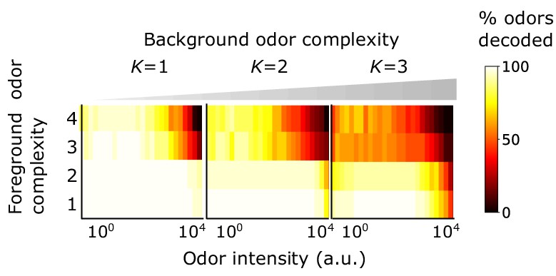
Benefits conferred by Weber-Fechner adaptation remain for a broader distribution of baseline adapted activity levels , now assumed to be ORN-dependent and chosen from a normal distribution. (A) Distribution of . (B) Decoding accuracy of foreground odors in the presence of background odors. .
Figure 3—figure supplement 3
Decoding accuracy for receptors with multiple binding sites.
Benefits conferred by Weber-Fechner adaptation remain for two binding sites per receptor. This might conceivably occur in insect olfactory receptors, heterotetramers consisting of 4 Orco/Or subunits that gate a central ion channel pathway (Butterwick et al., 2018). Plotted is the decoding accuracy of foreground odors in the presence of background odors. .
Figure 3—figure supplement 4
Preservation of restricted isometry property in CS shows how decoding accuracy is maintained by adaptation.
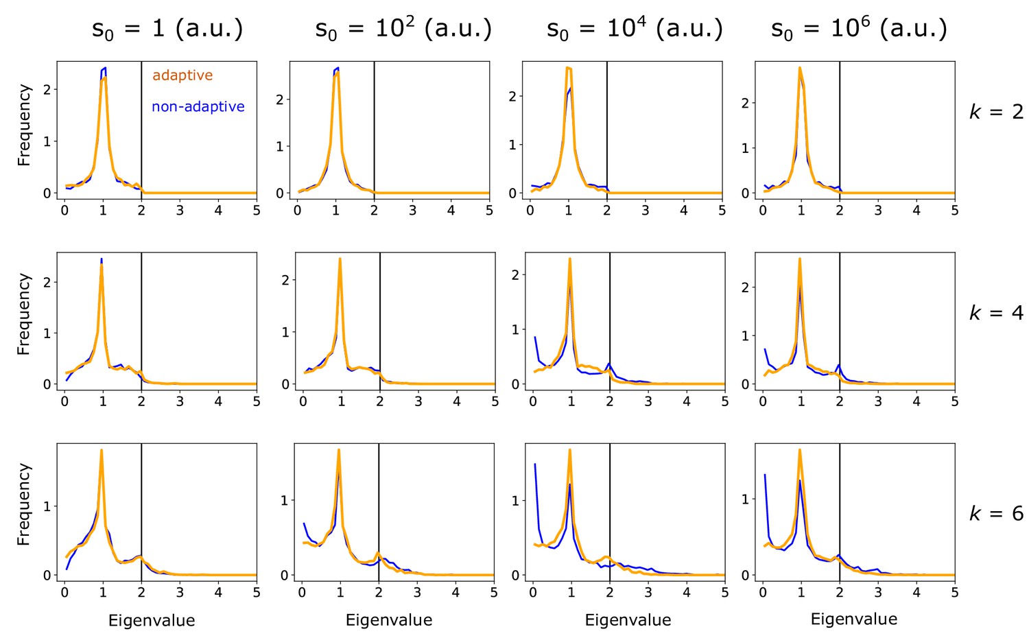
Eigenvalue distribution of , where is a submatrix of the column-normalized linearized ORN response matrix , evaluated at the linearization point . Note that is -sparse, but its components do not necessarily align with the columns chosen for the sub-matrix. Eigenvalues are calculated for the adaptive (orange) and non-adaptive (blue) systems, for 1000 randomly chosen linearization points and submatrices. Plots are arranged for various odor sparsities (by row) and odor intensities (by column). The restricted isometry property is satisfied when the eigenvalues lie between 0 and 2 (black vertical line), and is more strongly satisfied the more centered the distribution is around unity. The increase in near-zero eigenvalues for the non-adaptive system at higher odor complexities and intensities (lower right plots) indicates the weaker fulfillment of the restricted isometry property for these signals, and leads to higher probability of failure in compressed sensing signal reconstruction. .
Figure 3—figure supplement 5
Odor decoding accuracy using the iterative hard thresholding algorithm for nonlinear compressed sensing.
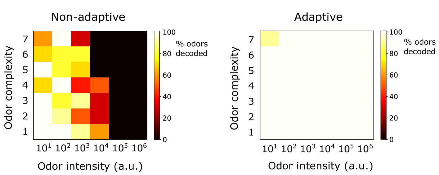
Decoding of odor signals (no background odors) using the IHT algorithm (Blumensath and Davies, 2009b; Blumensath, 2013) qualitatively reproduces the results from the main text, which used traditional CS with background linearization. In the adaptive case, IHT actually exhibits superior accuracy to traditional CS, although IHT demands more compute time. The results here show odor decoding accuracy for sparse odor signals of given complexity and intensity, averaged over 10 distinct identities. The iterative algorithm was initialized at and run forward until was stationary, or 10,000 iterations were reached. Step size in Equation 22 was set to . At each step, the linearized response used in determining ( in Equation 22) was evaluated at the result of th iteration, . IHT also requires an assumption on the number of components in the mixture (which defines in Equation 22); here, that was set to twice the actual sparsity of true signal.
Figure 3—figure supplement 6
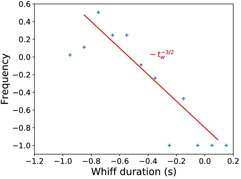
Whiff duration distribution in naturalistic stimulus.
Distribution of whiff durations in naturalistic stimulus, compared to the theoretical prediction (Celani et al., 2014).
Figure 4 with 1 supplement
Effect of front-end adaptation on primacy coding.
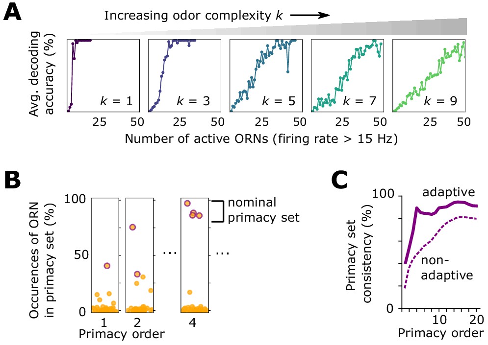
(A) Decoding accuracy as a function of the number of active ORNs, for different odor complexities. The primacy set consists of those ORNs required to be active for accurate decoding. (B) Frequency of particular ORNs in primacy sets of an odor placed atop different backgrounds. Individual plots show, for given primacy order , the percentage of backgrounds for which the primacy set of odor A contains a given ORN (dots). Those with purple borders are the most highly occurring – that is a nominal background-invariant primacy set for odor A. Points are jittered horizontally for visualization. (C) Consistency of primacy sets across backgrounds, as a function of , for the adaptive (solid) and non-adaptive (dashed) system. Consistency is defined as the likelihood that an ORN in the nomimal primacy set appears in any of the individual background-dependent primacy sets, averaged over the nominal set (average of the y-values of the purple dots in B). 100% consistency means that for all backgrounds, the primacy set of odor (A) is always the same ORNs.
Figure 4—figure supplement 1

Additional results for primacy coding in the adaptive ORN model.
Additional results pertaining to the primacy coding hypothesis. (A) Percent of active ORNs required for 75% accuracy of a steep sigmoidal odor step, as a function of odor step intensity and odor complexity. For low complexities, a primacy set of fewer ORNs may be sufficient to decode the full odor signal; for higher complexities, the entire ORN repertoire is required. (B) In the primacy coding hypothesis, the primacy set is realized sooner for stronger odor signals, so odors are decoded earlier in time, resulting in a perceptual time shift with increasing odor concentration (Wilson et al., 2017). We also find this shift in our compressed sensing decoding framework (right plot), which rises monotonically with step height for various odor complexities, in agreement with primacy coding. (C) The consistency of a primacy code across changes in background odor concentration, in a system with Weber Law adaptation. We calculate the primacy set for odor A (step odor; black) in the presence of either a weak, medium, or strong background (dotted lines; 1x, 10x, 100x a.u.), assuming the system has adapted its response to the background as described in the main text. Averaged across odor A identities, primacy sets for odor A when in the 1x background are nearly identical to those when odor A is in the 10x background (right plot; yellow). The same holds true when comparing the 1x and 100x backgrounds, for sufficiently large primacy order, above eight or so right plot; purple). This indicates that Weber Law adaptation preserves primacy codes across disparate environmental conditions.
Figure 5 with 1 supplement
Front-end adaptation enhances odor recognition by the Drosophila olfactory circuit.
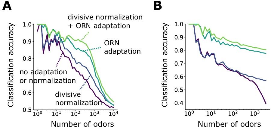
(A) Accuracy of linear classification by odor identity, as a function of the number of distinct odor identities classified by the trained network (concentrations span 4 orders of magnitude), in systems with only ORN adaptation, only divisive normalization, both or neither. (B) Same as (A) but now classifying odors by valence. Odors were randomly assigned valence. For a given odor identity, the valence is the same for all concentrations.
Figure 5—figure supplement 1
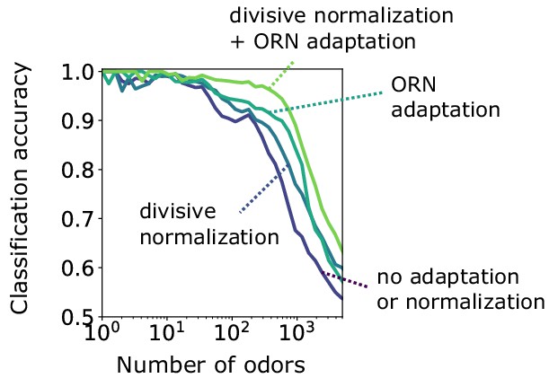
Binary classification for odors whose concentrations span a narrow range of concentration.
Accuracy of binary classification by odor valence, for odors whose concentrations span a narrow range of concentrations (1 order of magnitude). Accuracy is plotted as a function of the number of distinct odor identities classified by the trained network, in systems with only ORN adaptation, only divisive normalization, both or neither. Decoding gains conferred by divisive normalization and/or ORN adaptation are much smaller than when odors span a much larger range of concentrations, as shown in the main text.
Additional files
-
Transparent reporting form
- https://doi.org/10.7554/eLife.45293.017
Download links
A two-part list of links to download the article, or parts of the article, in various formats.
Downloads (link to download the article as PDF)
Open citations (links to open the citations from this article in various online reference manager services)
Cite this article (links to download the citations from this article in formats compatible with various reference manager tools)
Front-end Weber-Fechner gain control enhances the fidelity of combinatorial odor coding
eLife 8:e45293.
https://doi.org/10.7554/eLife.45293


