Polar pattern formation induced by contact following locomotion in a multicellular system
- Laboratory for Physical Biology, RIKEN Center for Biosystems Dynamics Research, Japan
- Mechanobiology Institute, National University of Singapore, Singapore
- Universal Biology Institute, University of Tokyo, Japan
- Faculty of Life and Environmental Sciences, University of Tsukuba, Tennodai, Japan
Figures
Figure 1 with 1 supplement
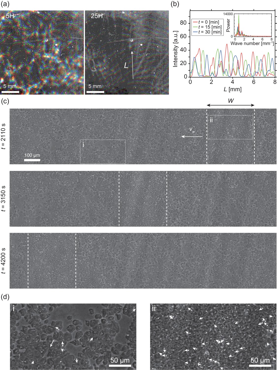
Segregation of cell density and formation of bands in non-chemotactic D. discoideum KI cell.
(a) The density profile of three time points with a time interval of 15 min indicated by color-coding (red t = 0 min, green 15 min, blue 30 min). Brighter color indicates higher density. Five (left) and 25 (right) hours after incubation. See also Video 1. (b) The intensity profile along the line indicated in (a), showing a periodic distribution of high-density regions. The inset shows a power spectrum of the intensity profile, indicating that the spatial interval was about 1 mm. (c) Time evolution of phase-contrast image of high-density region (dotted lines) at t = 2110, 3150, 4200 s, respectively. The time points correspond to that in Video 2. (d) High magnification images of low-density region (i) and high-density region (ii). Arrows indicate the migration directions of cells.
-
Figure 1—source data 1
Statistics of traveling bands.
This file contains width, traveling speed, average cell speeds inside and outside of the bands, order parameter value and number of trajectories analyzed of 10 independent experiments.
- https://cdn.elifesciences.org/articles/53609/elife-53609-fig1-data1-v3.xlsx
Figure 1—figure supplement 1
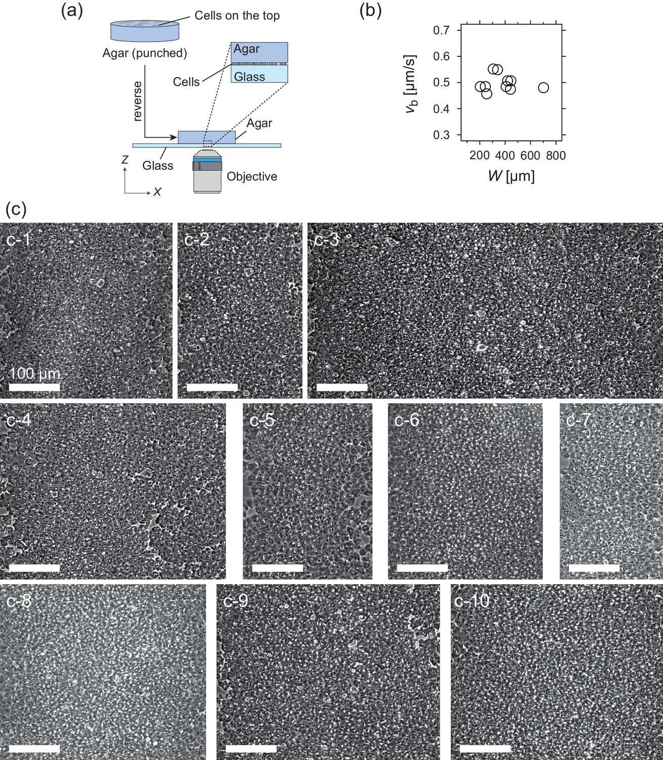
Experimental setup and properties of traveling band.
(a) Experimental setup for the microscopic observation of the polar pattern formation. (b) Relationship between the propagation speed vb and size of the wave W. (c) Snapshots of propagating band. The number of waves studied is N = 10. (c-1) W = 340 µm; (c-2) W = 244 µm; (c-3) W = 702 µm; (c-4) W = 445 µm; (c-5) W = 255 µm; (c-6) W = 306 µm; (c-7) W = 204 µm; (c-8) W = 408 µm; (c-9) W = 442 µm; (c-10) W = 419 µm. Source data for (b) is available in Figure 1—source data 1.
Figure 2
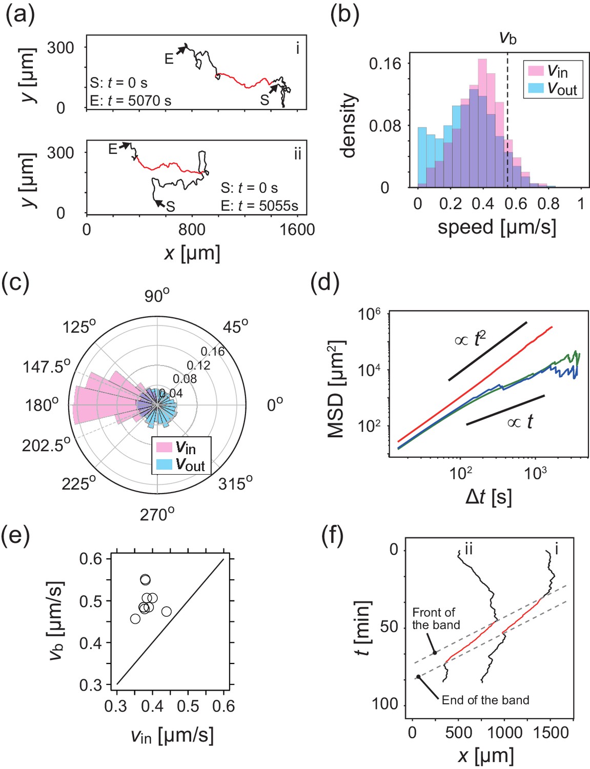
Analysis of single cell migrations inside and outside the band.
(a) Trajectories of single cells inside (red) and outside (black) the band taken every 15 s. These trajectories were taken from the data shown in Figure 1c. (b,c) The distributions of the migration speed (b) and migration direction (c) inside (pink) and outside (blue) the band shown in Figure 1c. The number of trajectories analyzed is N=35. In Figure 1c, the average of migration direction inside the band (pink) was 176.2 degrees and the standard deviation was 42.7 degrees. (d) Mean squared displacement (MSD) of cell motions inside the band (red), before entering the band (green) and after leaving the band (blue) (e) Scatter plot of the band speed against the cell speed within the band. The number of bands investigated is . Trajectory data and traveling band position are available in Figure 2—source datas 1 and 2. Source data for (e) is available in Figure 1—source data 1. (f) Spatiotemporal plot of trajectories shown in a. The x coordinates of trajectories (horizontal axis) are plotted against time (vertical axis). The front and back of traveling band are shown by dotted lines.
-
Figure 2—source data 1
Trajectory data of 35 cells in the experiment shown in Figure 1c.
- https://cdn.elifesciences.org/articles/53609/elife-53609-fig2-data1-v3.csv
-
Figure 2—source data 2
Front and end positions of band as functions of time in the experiment shown in Figure 1c.
- https://cdn.elifesciences.org/articles/53609/elife-53609-fig2-data2-v3.csv
Figure 3 with 4 supplements
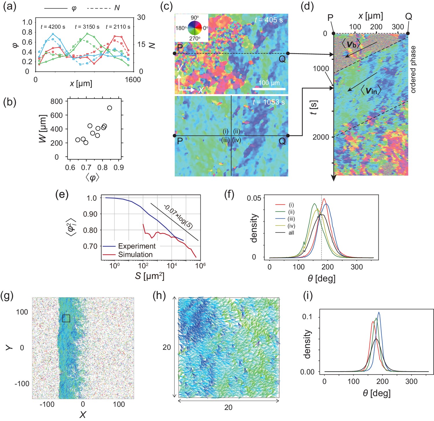
Analysis of heterogeneity within the ordered phase.
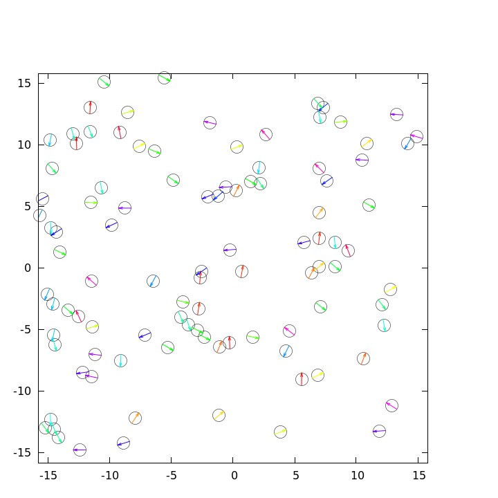
(a) Spatial profile of the local polar order parameter (solid lines) and the number of beads in the intervals (dotted lines) in Figure 1c. (b) Scatter plot of band width against polar order parameter within the band region. The number of bands studied is . (c) Optical flow images in the front region of a band t=405 (top) and within the band t=1083 (bottom). See also Video 3. (d) Kymograph of the optical flow image along the line PQ shown in (c) (top). The arrows indicate the average velocity of band and the average cell speed . (e) Size-dependent squared local order parameter plotted against the area S for the data shown in (c). (f) Probability distribution function (pdf) of the migration direction within the band region obtained by averaging the pdfs of the sequential 150 frames in Video 3. The pdfs (i)-(iv) are obtained in the regions (i)-(iv) in (c) (bottom), respectively. Average pdf is shown by the black line (the mean is 178.1 degrees and the standard deviation is 31.2 degrees). (g) Snapshot of simulation result showing a polar ordered phase as a propagating band in the background of disordered phase. The color code indicates the migration direction of individual particle as shown in (c). See also Video 8. (h) Magnification of squared area shown in g. The size of area (20x20) is comparable to the whole area shown in (c). Each arrow indicates the direction of polarity. (i) Probability distribution function of the migration direction within the band region in the simulation (red, green and blue lines). For the choice of ROI, see Materials and methods. Average pdf is shown by the black line. Source data for (b) is available in Figure 1—source data 1.
Figure 3—figure supplement 1
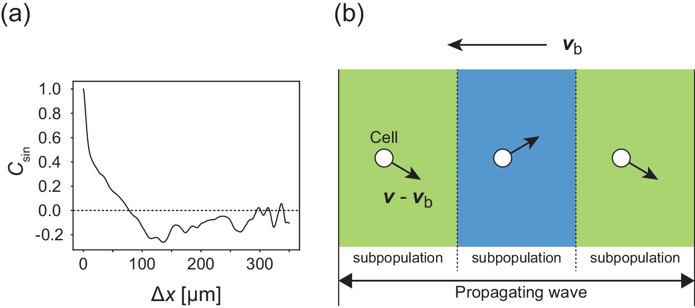
Internal structure within a traveling band.
(a) Autocorrelation function of transverse motion with respect to the wave propagation direction , indicating that the typical width of the stripe was around 125 µm. (b) Illustration of the cell migration within the formed stripes in the co-moving frame. Arrows from cells indicate the direction of motion relative to the velocity vector of wave propagation.
Figure 3—figure supplement 2
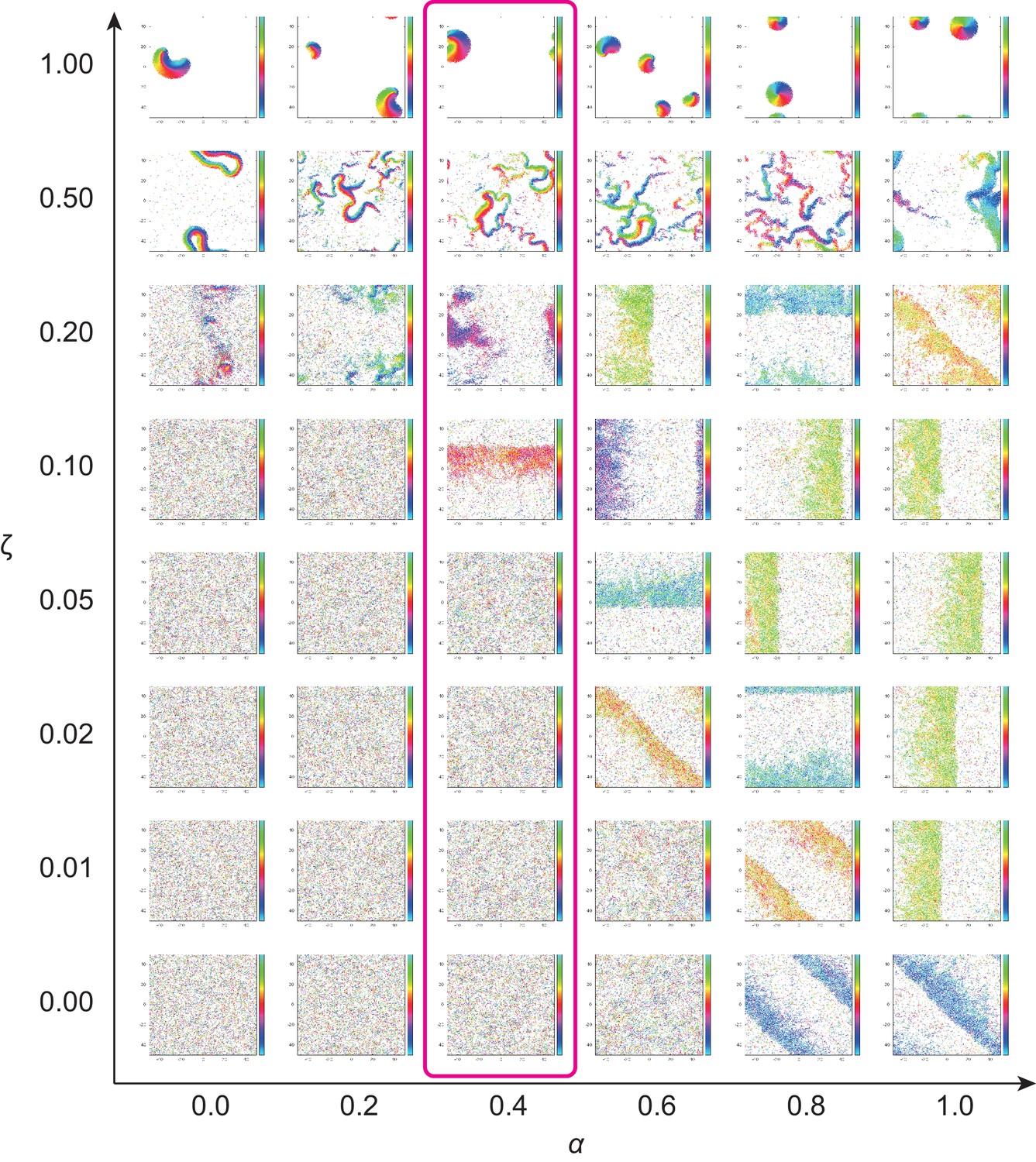
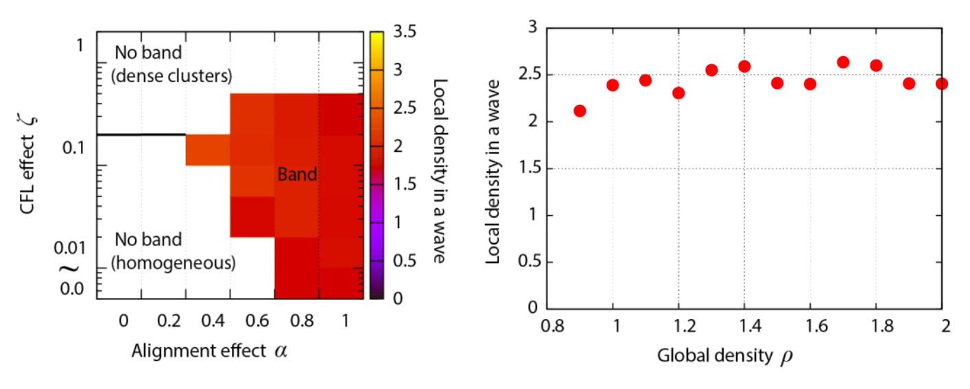
Phase diagram of the agent-based simulation for changes of CFL α and the alignment effect ζ.
A region where α = 0.4 is surrounded by the pink line.
Figure 3—figure supplement 3

Analyses of heterogeneityin the numerical simulations.
(a, b) The regions of interest used in the analyses (bright yellow) within the wave (dark yellow) for (a) CFL-induced and (b) alignment-induced waves, respectively. Analysis method to pick up these ROIs is found in Materials and methods. (c, d) Pdfs of the migration direction within the wave region with the top eight and nine peak probability densities for (c) CFL-induced and (d) alignment-induced waves, respectively. (e,) Typical pdfs for alignment-induced waves extracted from (d).
Figure 3—figure supplement 4

Analysis of internal structure from individual cell trajectories.
(a) Spatiotemporal plot of trajectories (solid line) studied in Figure 2 and temporal average of migration direction in each lattice (color). Intervals of the lattice in time and x position are 60 s and 20 µm, respectively. In the lattice without color, there was no trajectory. (b) Plot of temporal average of migration direction at a given x position (left). Definition of x0, x1. (right) The temporal average of migration direction was obtained by averaging the angle values in each rectangle.
Figure 4 with 1 supplement
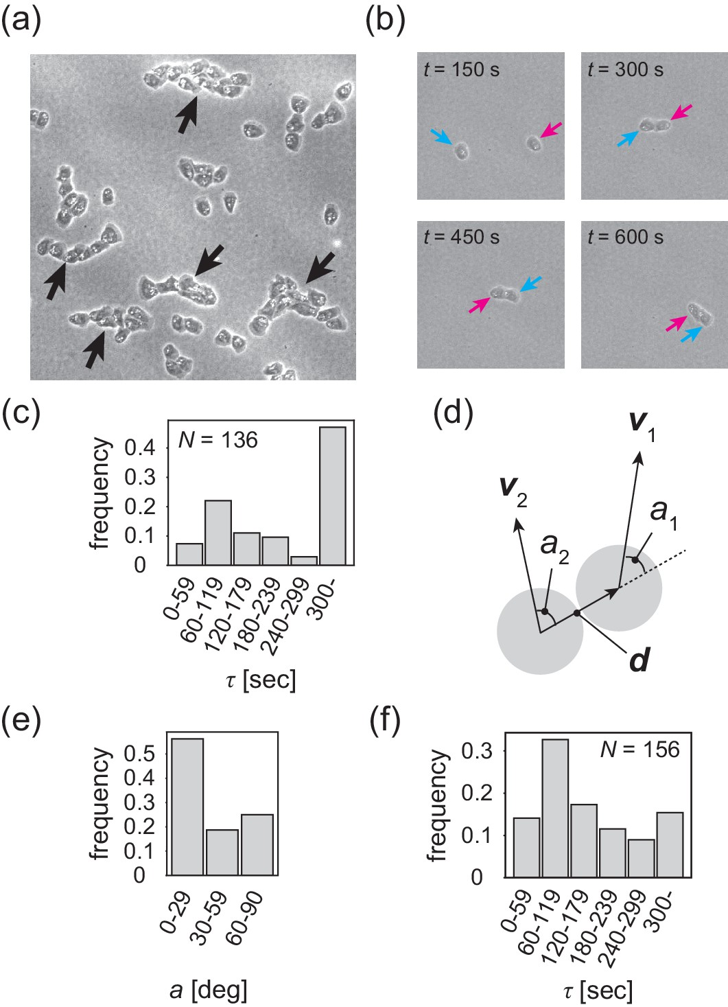
Contact following locomotion responsible for band propagation.
(a) Snapshot of the contact following locomotion. See also Video 4. (b) Representative time evolution of collision of two cells. Colored arrows represent the same cell. See also Video 5. (c) Histogram of the duration of two cell contacts for KI cell (control). (d) Schematic of angle (), which is the angle of the velocity vector () with respect to the vector connecting two cell centers. Then, the angle is obtained as the angular average of and , that is . (e) Histogram of the angle for the KI cells that contact each other for >300 s. (f) Histogram of the duration of two cell contacts for the tgrb1 null mutant. Source data for (c) and (f) are available in Figure 4—source datas 1 and 2.
-
Figure 4—source data 1
Source data of duration of two cell contacts for KI cell shown in Figure 4c.
- https://cdn.elifesciences.org/articles/53609/elife-53609-fig4-data1-v3.csv
-
Figure 4—source data 2
Source data duration of two cell contacts for tgrb1 mutant cell shown in Figure 4f.
- https://cdn.elifesciences.org/articles/53609/elife-53609-fig4-data2-v3.csv
Figure 4—figure supplement 1
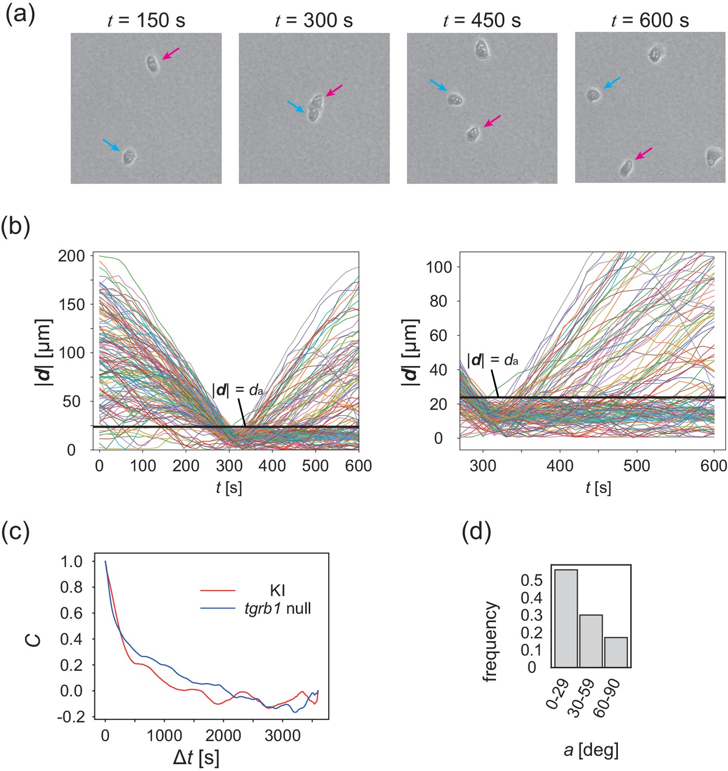
Collision analysis and locomotive activity of KI and tgrB1 mutant cells.
(a) Another example of time evolution of collision of two cells. (b) Time series of distance between two cells |d|. Each line is a data obtained from different cell pairs. Black horizontal line means . Time series of |d| after the collision (t = 300 s) is magnified in the right panel. (c) The velocity auto-correlation functions of the isolated cells. Red line: KI cell. Blue line: tgrb1 null mutant. (d) Histogram of the CFL angle a for the tgrb1 null mutant cells that contact each other for >300 s.
Author response image 1

Author response image 2
Author response image 3
Videos
Video 1
Macroscopic observation of the propagating bands.
The video was taken every 15 min for 28.5 hr. Video acceleration: 11400 × real time.
Video 2
Microscopic observation of the propagating bands.
The video was taken every 15 s for 1.66 hr. Video acceleration: 230 × real time.
Video 3
Propagating band with overlaying the coloring based on the optical flow analysis.
The video was taken every 3 s for 39.5 min. Video acceleration: 151 × real time.
Video 4
Migration of the KI cells in the low-density region.
The video was taken every 15 s for 2 hr. Video acceleration: 378 × real time.
Video 5
A binary collision of the KI cells in the low-density assay.
The video was cropped from the video of the low-density assay with a length of 10.25 min. Video acceleration: 153 × real time.
Video 6
Macroscopic observation of the population of tgrb1 null mutant.
The video was taken every 15 min for 28.5 hr. Video acceleration: 11400 × real time.
Video 7
Microscopic observation of the population of tgrb1 null mutant.
The video was taken every 15 s for 1.25 hr. Video acceleration: 225 × real time.
Video 8
Propagating band formation generated in the agent-based simulation.
The color code indicates the migration direction of individual particle as shown in Figure 3c. Arrows indicate the direction of polarity.
Tables
Key resources table
| Reagent type (species) or resource | Designation | Source or reference | Identifiers | Additional information |
|---|---|---|---|---|
| Cell line (Dictyostelium discoideum) | KI-5 | National BioResource Project Cellular slime molds | NBRP ID: S00058 | Available in National BioResource Project Cellular slime molds (https://nenkin.nbrp.jp) |
Additional files
Download links
A two-part list of links to download the article, or parts of the article, in various formats.
Downloads (link to download the article as PDF)
Open citations (links to open the citations from this article in various online reference manager services)
Cite this article (links to download the citations from this article in formats compatible with various reference manager tools)
Polar pattern formation induced by contact following locomotion in a multicellular system
eLife 9:e53609.
https://doi.org/10.7554/eLife.53609


