DeepFRET, a software for rapid and automated single-molecule FRET data classification using deep learning
- Department of Chemistry and Nanoscience Centre, University of Copenhagen, Denmark
- Structural Molecular Biology Group, Novo Nordisk Foundation Centre for Protein Research, Faculty of Health and Medical Sciences, University of Copenhagen, Denmark
- Niels Bohr Institute, University of Copenhagen, Denmark
- Novo Nordisk Foundation Centre for Protein Research, Faculty of Health and Medical Sciences, University of Copenhagen, Denmark
Figures
Figure 1 with 11 supplements

Overview of smFRET evaluation and analysis using DeepFRET.
(a) Cartoon of the typical heterogeneous data acquired in smFRET experiments. Varying criteria for data selection for downstream analysis may yield different structural and kinetic information. (b) Screenshots of the provided standalone software that integrates deep learning and reduces the selection to a single-user-adjustable criterion: the DEEP FRET confidence threshold. The simple and intuitive GUI integrates all the features of our approach for rapid traces extraction from raw images to filtering of traces based on the predicted classification, treatment of smFRET data to extraction of publication-quality figures. (c) End-to-end sequence classification of smFRET traces by deep learning. Raw signals of donor-donor, donor-acceptor, and acceptor-acceptor intensities in the form of ASCII files can also be loaded with the DeepFRET software. The pre-trained DNN will classify individual frames into one of six different categories: bleached, static smFRET, dynamic smFRET, aggregate, noisy, and scrambled. A final smFRET confidence score is calculated, depending on each of the categories, that is used for threshold.
-
Figure 1—source data 1
Data underlying Figure 1—figure supplements 3, 4 , and 7.
- https://cdn.elifesciences.org/articles/60404/elife-60404-fig1-data1-v1.zip
Figure 1—figure supplement 1
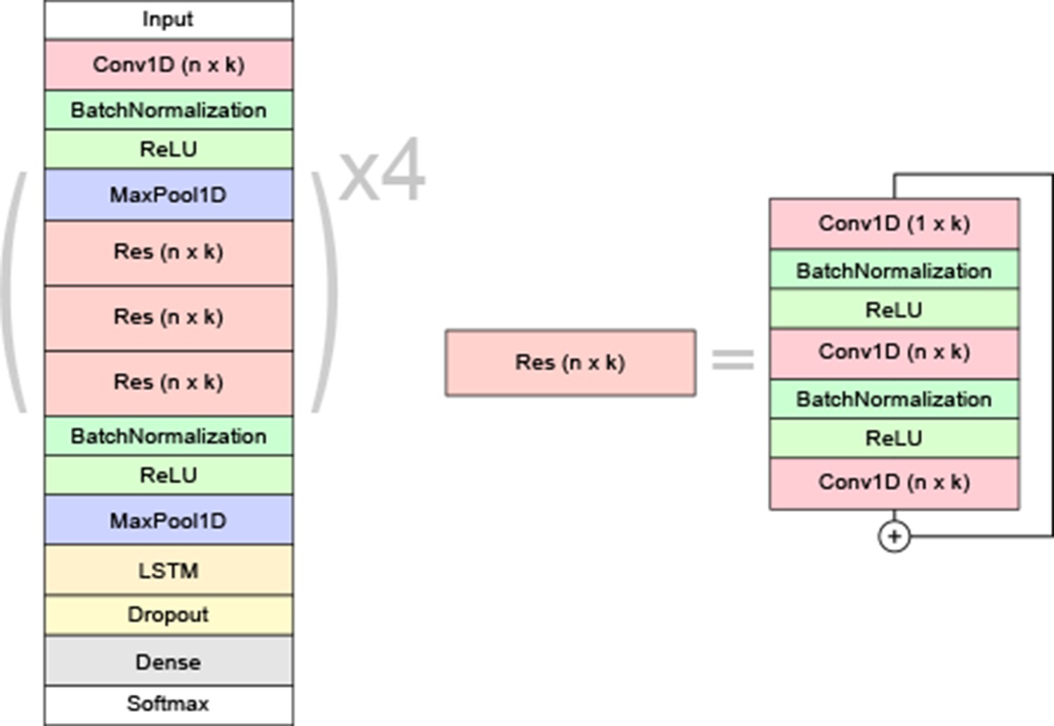
Schematic overview of the neural network model architecture.
Each residual block (Res) is made up of 1D convolutional filters of size n × k with batch normalization and ReLU activations in between. The initial convolution after the input layer has the same hyper-parameters as the first residual block. A 1 × k convolution is added in each bottleneck unit for efficiency. The ‘+’ symbol denotes a skip-connection, where the residual block’s input is added to its output. The final convolved output goes to a bidirectional long short-term memory (LSTM) layer. For each frame, the outputs are distributed among the different classes by a dense layer with softmax activation.
Figure 1—figure supplement 2
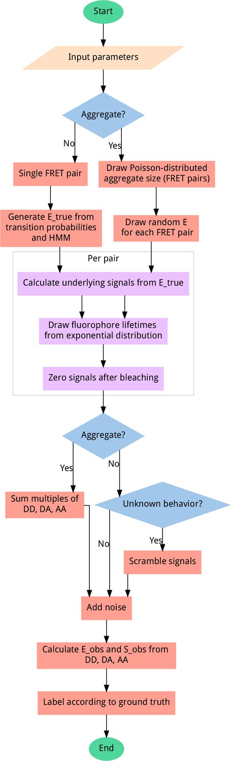
Data generator algorithm overview.
To generate unbiased distributions of smFRET traces, most steps include randomization, sampling from uniform distributions (except for bleaching probability, which follows an exponential distribution) for the given input parameter ranges. User-adjustable parameters include the probability of aggregation, fluorophore blinking, bleaching, and more. All output data is automatically sequence-annotated with the ground truth behavior, for supervised machine learning. A scrambling probability is used to generate a fraction of heavily distorted data to improve model robustness and prevent misclassification of data containing artifacts.
Figure 1—figure supplement 3
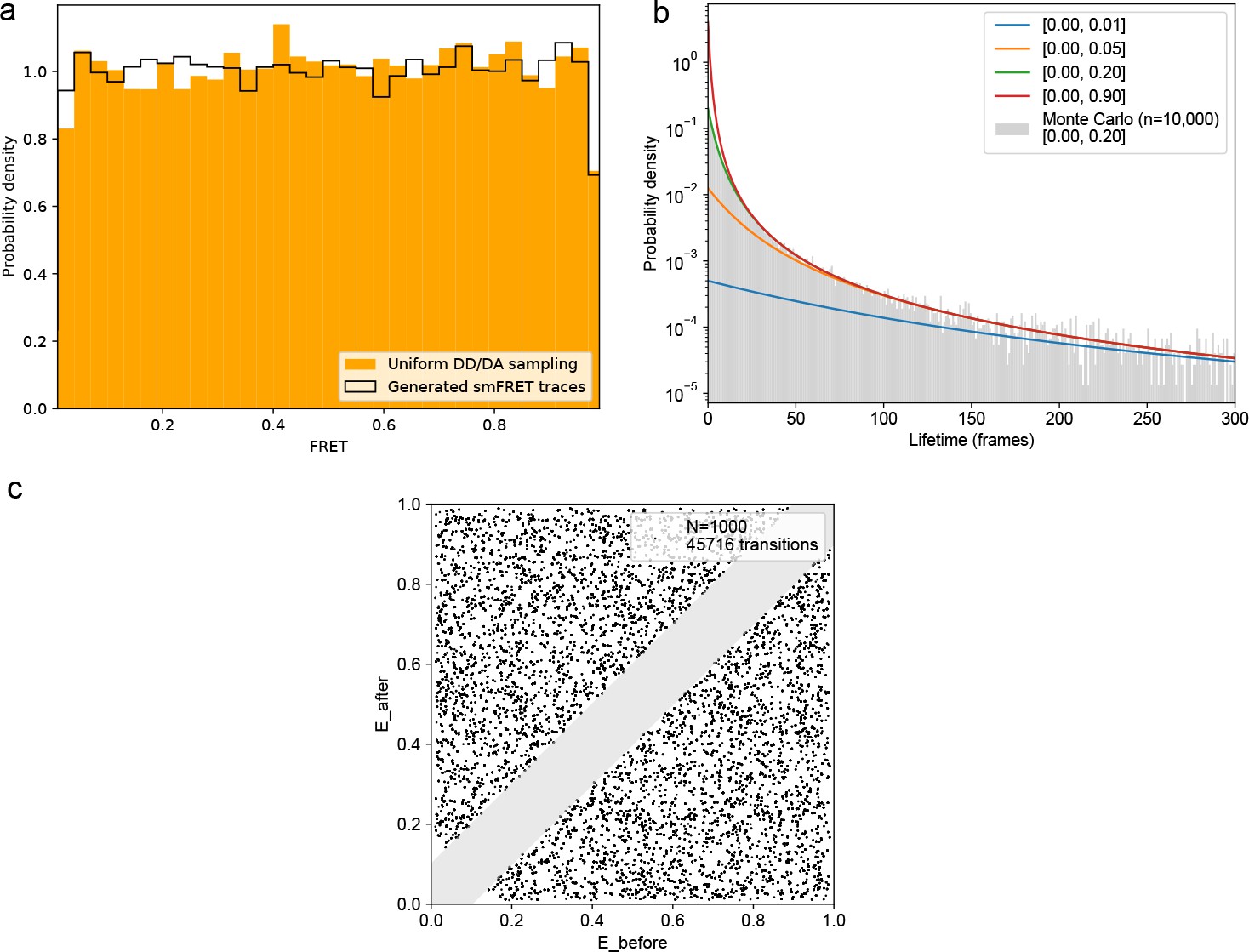
FRET values, dynamic FRET state lifetimes, and transition pathways are uniformly sampled for all ground truth smFRET traces.
(a) smFRET traces were generated with 1–4 randomly defined FRET states with the same transition probabilities as used for model training. Comparing FRET calculated from uniformly sampled donor/acceptor intensities between 0 and 1 reveals identical, uniform distributions. (b) Theoretical lifetime distributions for various ranges of sampled transition probabilities. The lifetime distribution follows an evenly weighted average over the exponential decays for each possible number of FRET states and transition probabilities. A Monte Carlo simulation derived by sampling transition probabilities uniformly between 0 and 0.2, as in the training data, on n = 10,000 traces sampling from 2 to 4 FRET states is in agreement with the underlying model. (C) Transition density plot displaying the idealized transitions of n = 1000 simulated FRET traces. A minimum distance of 0.1 FRET between states was used, as in the training data, to distinguish actual transitions from noise fluctuations, hence the grayed out diagonal. The simulated training data does not introduce any bias in the model training.
Figure 1—figure supplement 4

Noise threshold for simulated data.
(a) To tune the accepted noise level for our deep learning model, we simulated 200 smFRET traces with a single state at 0.5 FRET, with varying noise levels. (b) At a noise level of 0.25, the distributions in (a) could no longer be considered normal, using a D’Agostino-Pearson test for normality (p<0.05).
Figure 1—figure supplement 5
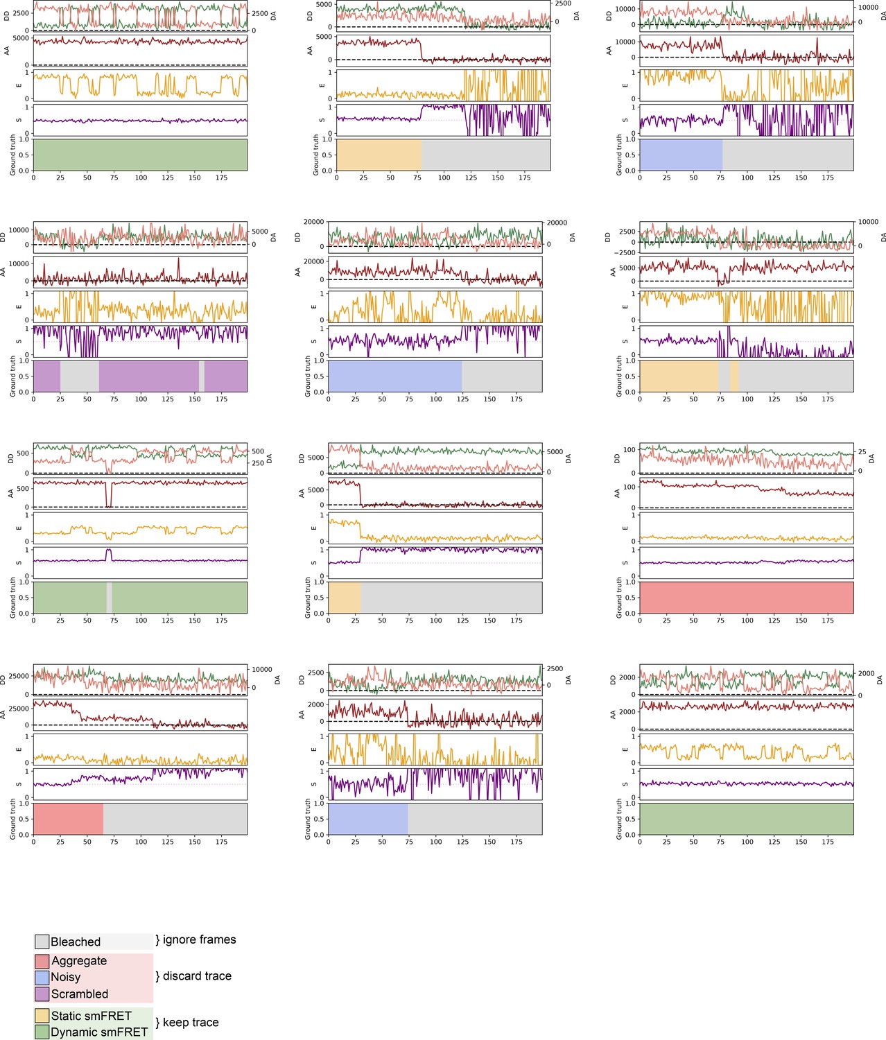
Examples of randomly generated traces.
Randomly generated traces, corresponding to each of the six defined categories, shown with raw signals, E (FRET), and S (stoichiometry). The color code in the bottom panel corresponds to the frame-level ground truth labeling of each trace.
Figure 1—figure supplement 6
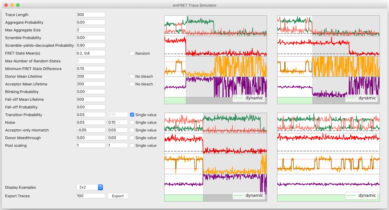
Trace simulator interface.
To facilitate fast and easy experimentation of any kind on smFRET traces, the DeepFRET GUI includes a visual trace simulator with ground-truth labels associated with every trace. The traces can be exported to ASCII or DAT and used for all kinds of statistical procedures.
Figure 1—figure supplement 7
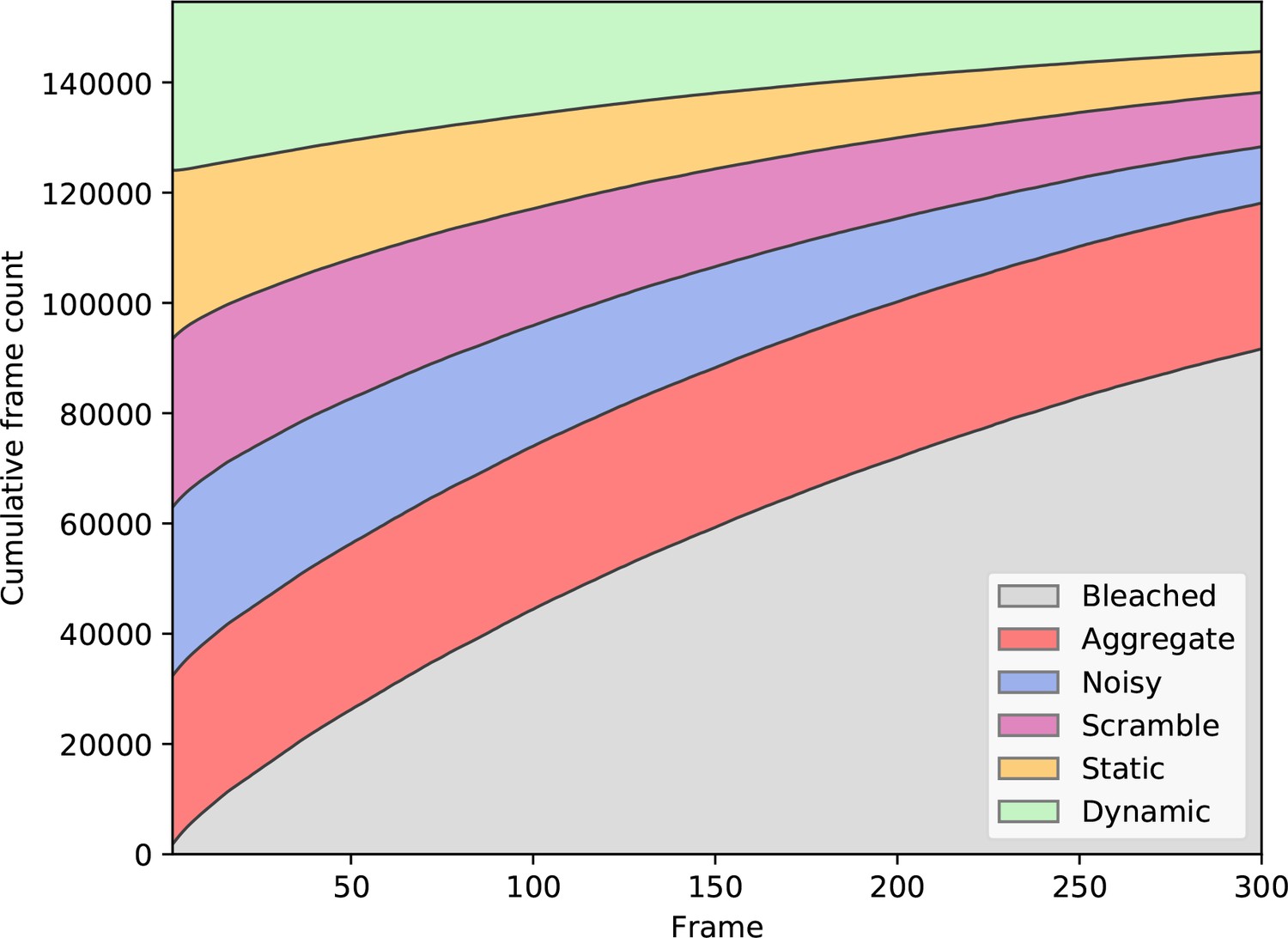
Training label dependence on the frame number.
The distribution of labels for all frames in the training dataset, after balancing classes based on the first frame. The ‘bleaching’ label is excluded from balancing, as it occurs in most of the generated traces, due to photobleaching.
Figure 1—figure supplement 8
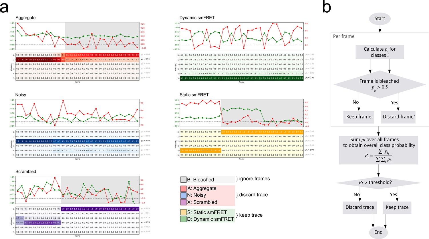
Calculation of confidence score from model predictions.
(a) Short toy-examples of selected traces for each category and the corresponding frame-wise predictions used for calculating confidence scores. The color code corresponds to classified behavior. All bleached data points (marked with gray in the trace) are excluded from the confidence score calculation. (b) Step-by-step calculation of trace scores.
Figure 1—figure supplement 9
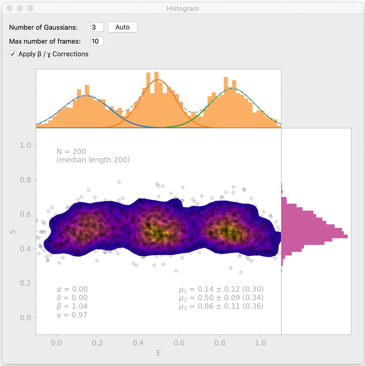
Histogram interface window.
DeepFRET includes a histogram window which automatically finds BIC-optimal Gaussian mixtures, and allows the user to test enter the number of Gaussians to include in a mixture model. The histogram interface also includes an option for β- and γ-correction. Data is simulated from DeepFRETs trace generator with three states with means 0.15, 0.5, and 0.85, as in Figure 2—figure supplement 2b.
Figure 1—figure supplement 10
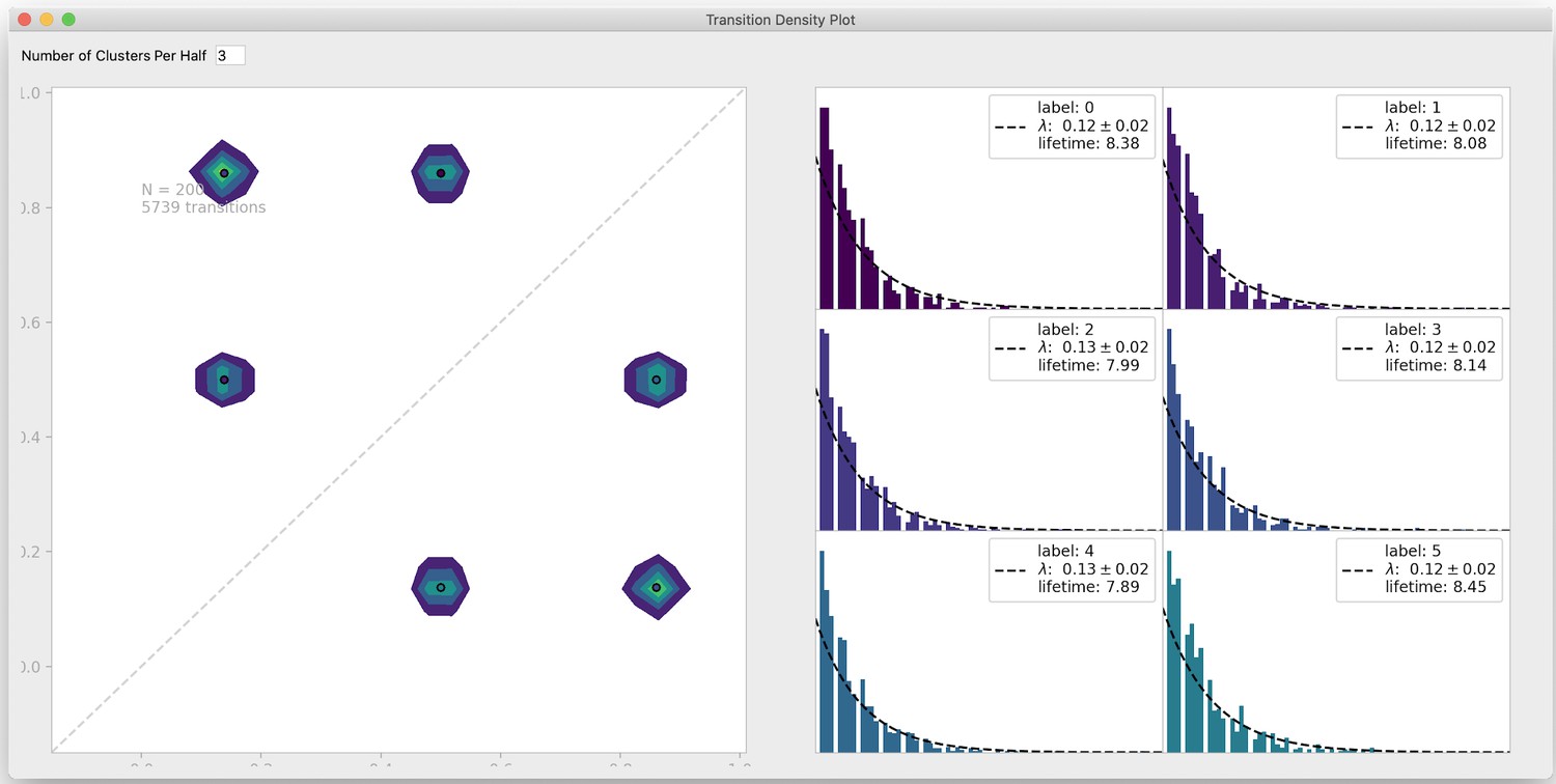
Transition density window.
To visualize transitions between FRET states, DeepFRET includes a window to fit exponential lifetime distributions of clusters in a transition density plot. The transition density interface also allows the user to test a different number of clusters for the transition density window. Data is simulated from DeepFRET’s trace generator with three states with means 0.15, 0.5, and 0.85, as in Figure 2—figure supplement 2b.
Figure 1—figure supplement 11
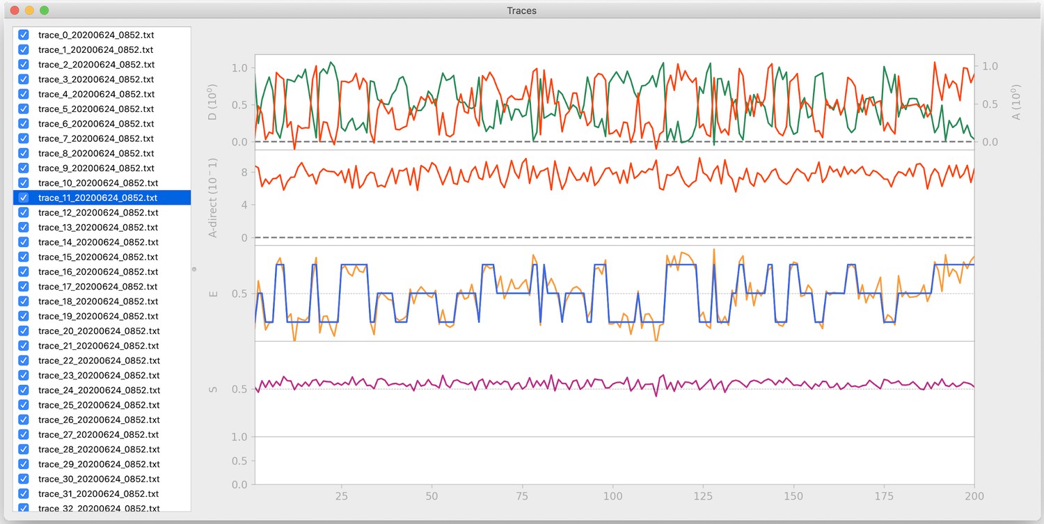
Traces window.
To provide direct visualization of the Hidden Markov modeling of smFRET traces, traces can be imported directly for HMM analysis using the commonly used pomegranate implementation of the Baum-Welch algorithm. The transitions from the traces window are used in the transition density window. Data is simulated from DeepFRET’s trace generator with three states with means 0.15, 0.5, and 0.85, as in Figure 2—figure supplement 2b.
Figure 2 with 3 supplements
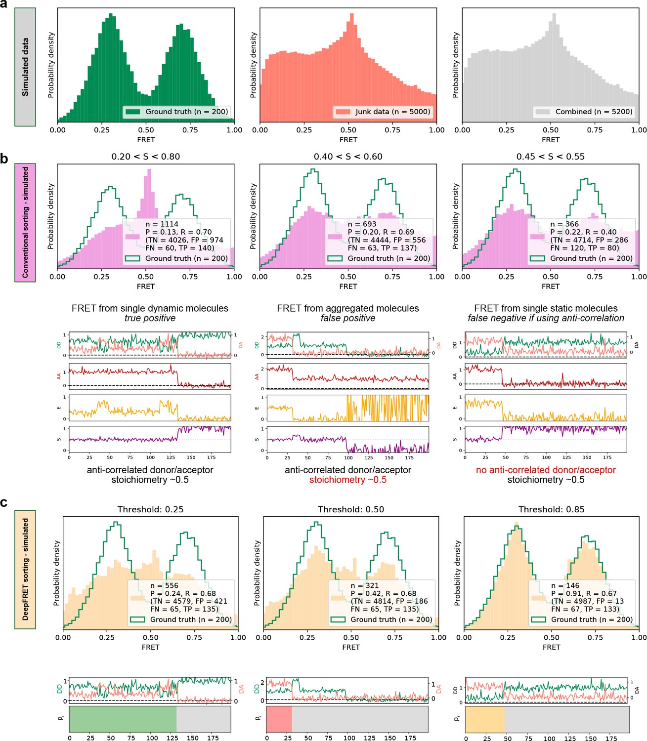
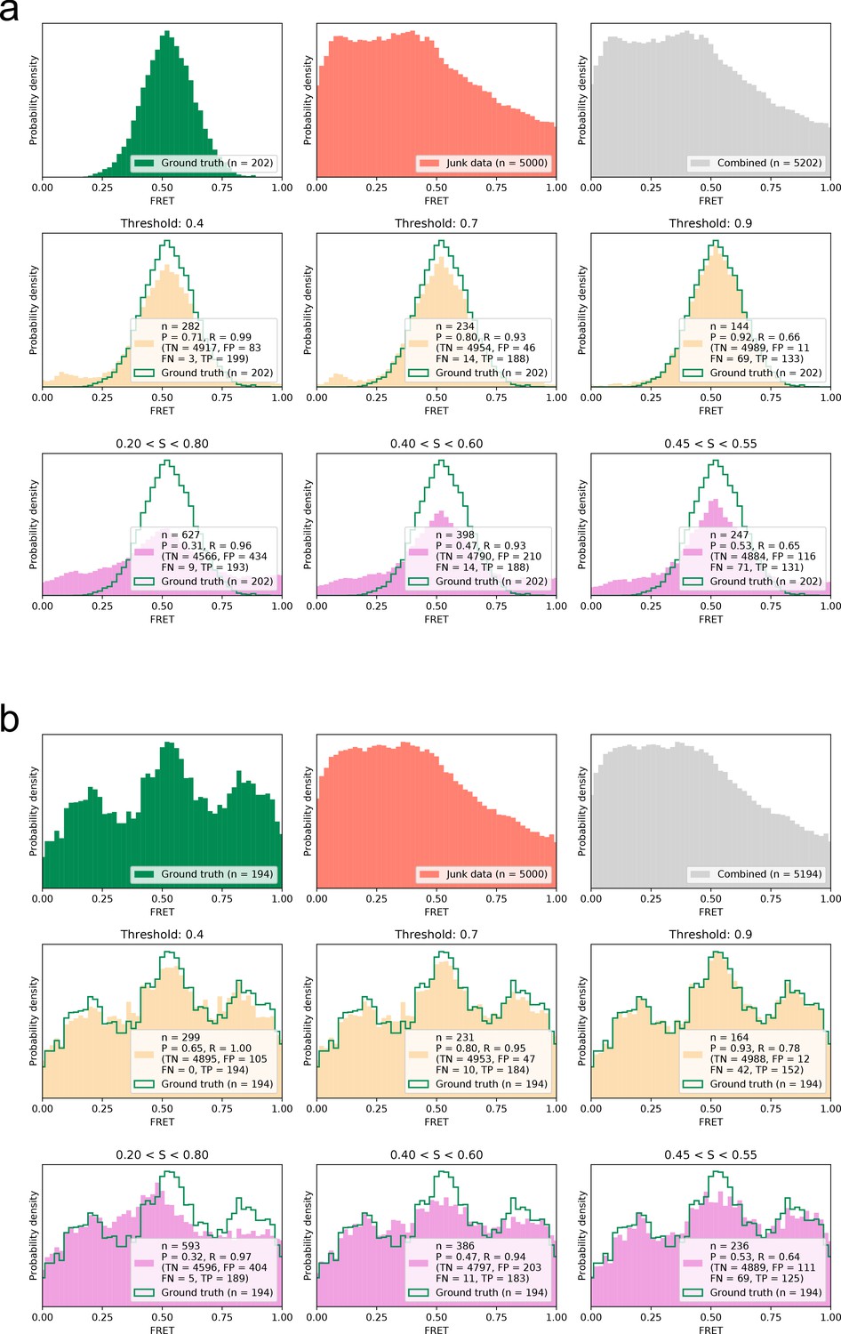
High quality FRET data evaluation.
(a) Simulated dynamic smFRET traces transitioning between FRET states 0.3 and 0.7 (left, ‘ground truth’) were mixed with a larger number of traces not showing smFRET (center). The overall distribution (right, ‘combined’) shows how the desired data can be drowned out in non-smFRET contaminant traces. The distribution would correspond to a raw distribution as extracted from raw image analysis of smFRET on low purity protein sample before any trace selection. (b) Automatic selection of data based on median stoichiometry, single-molecule intensity and bleaching. The number n designates the number of traces accepted by the model. Tightening the selection thresholds results in slight improvement of the poor overlap of the selected data with ground truth data, highlighting the need for a time-consuming and prone to potential cognitive biases human intervention. (c) Automatic classification of all traces of the combined set by DeepFRET, based only on the DeepFRET score threshold variation. Even at a low threshold DeepFRET selection follows the ground truth data. Increasing the score threshold further increases the fidelity of data selection. DeepFRET correctly assigns the dynamic, bleaching and aggregate behavior on the same smFRET traces as in (b) (see Figure 1—figure supplement 5 for more data). The single-user adjustable score threshold outperforms commonly used thresholds offering rapid, cross-lab reproducibility, and fully automatic data treatment. P: precision, R: recall, TN: true negatives, FP: false positives, FN: false negatives, TP: true positives.
-
Figure 2—source data 1
Data underlying Figure 2 and Figure 2—figure supplements 1–3.
- https://cdn.elifesciences.org/articles/60404/elife-60404-fig2-data1-v1.zip
-
Figure 2—source data 2
Data underlying Figure 2 and Figure 2—figure supplements 1–3.
- https://cdn.elifesciences.org/articles/60404/elife-60404-fig2-data2-v1.zip
-
Figure 2—source data 3
Data underlying Figure 2 and Figure 2—figure supplements 1–3.
- https://cdn.elifesciences.org/articles/60404/elife-60404-fig2-data3-v1.zip
-
Figure 2—source data 4
Data underlying Figure 2 and Figure 2—figure supplements 1–3 .
- https://cdn.elifesciences.org/articles/60404/elife-60404-fig2-data4-v1.zip
Figure 2—figure supplement 1
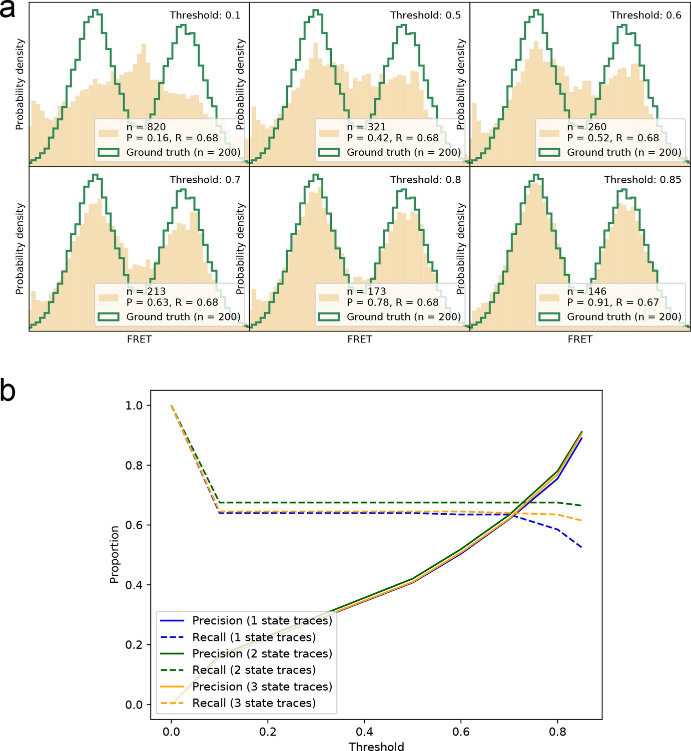
Precision-recall for correctly identifying smFRET traces at different thresholds.
(a) Visual display of recovered smFRET distributions for several thresholds for a 2-state system (same data as Figure 2). (b) The precision and recall are calculated for all thresholds on the datasets shown in Figure 2 and Figure 2—figure supplement 2. For 1-, 2-, and 3-state systems we find that a threshold around 0.8–0.9 provides the best trade-off between the two measures, in order to recover the underlying FRET distribution faithfully.
Figure 2—figure supplement 2
Comparison of smFRET distribution recovery by DeepFRET at different thresholds and semi-automated methodologies under various conditions in the absence of further human intervention.
In each of the figures (a) and (b); Top: ground truth distribution and distribution of randomly selected non-smFRET data from an external test set. Middle: Performance of DeepFRET sorting at different thresholds. Bleached frames were excluded from analysis in all cases. Bottom: Performance of sorting by semi-automated methodologies using common thresholds-based sorting at different thresholds. Classification metrics for smFRET trace detection are shown in the graph. (a) The performance, given a 1-state system centered at FRET mean value 0.5. (b) The performance, given a 3-state system centered at FRET mean values 0.15, 0.5, and 0.85.
Figure 2—figure supplement 3
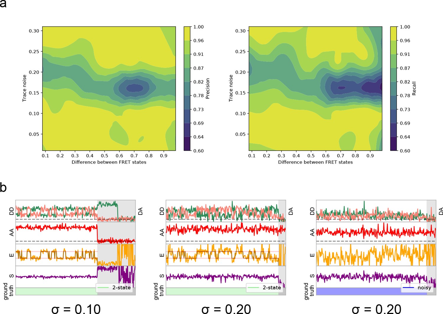
Relationship between model performance and noise level.
(a) 3D illustration of the precision or recall (pseudocolor) as a function of trace noise and the distance between FRET states for dynamic 2-state traces. Prediction accuracy is minimal at ~0.2 noise levels. At lower noise, the trace is accepted and correctly classified with an accuracy of >0.96, while at high noise levels the trace is accurately classified as non-FRET. (b) Examples of simulated dynamic traces used, with input simulation noise. At a high simulated noise level, only some traces are below the lower limit of acceptable noise, when measuring the per-state standard deviation of FRET of the final output trace.
Figure 3 with 1 supplement
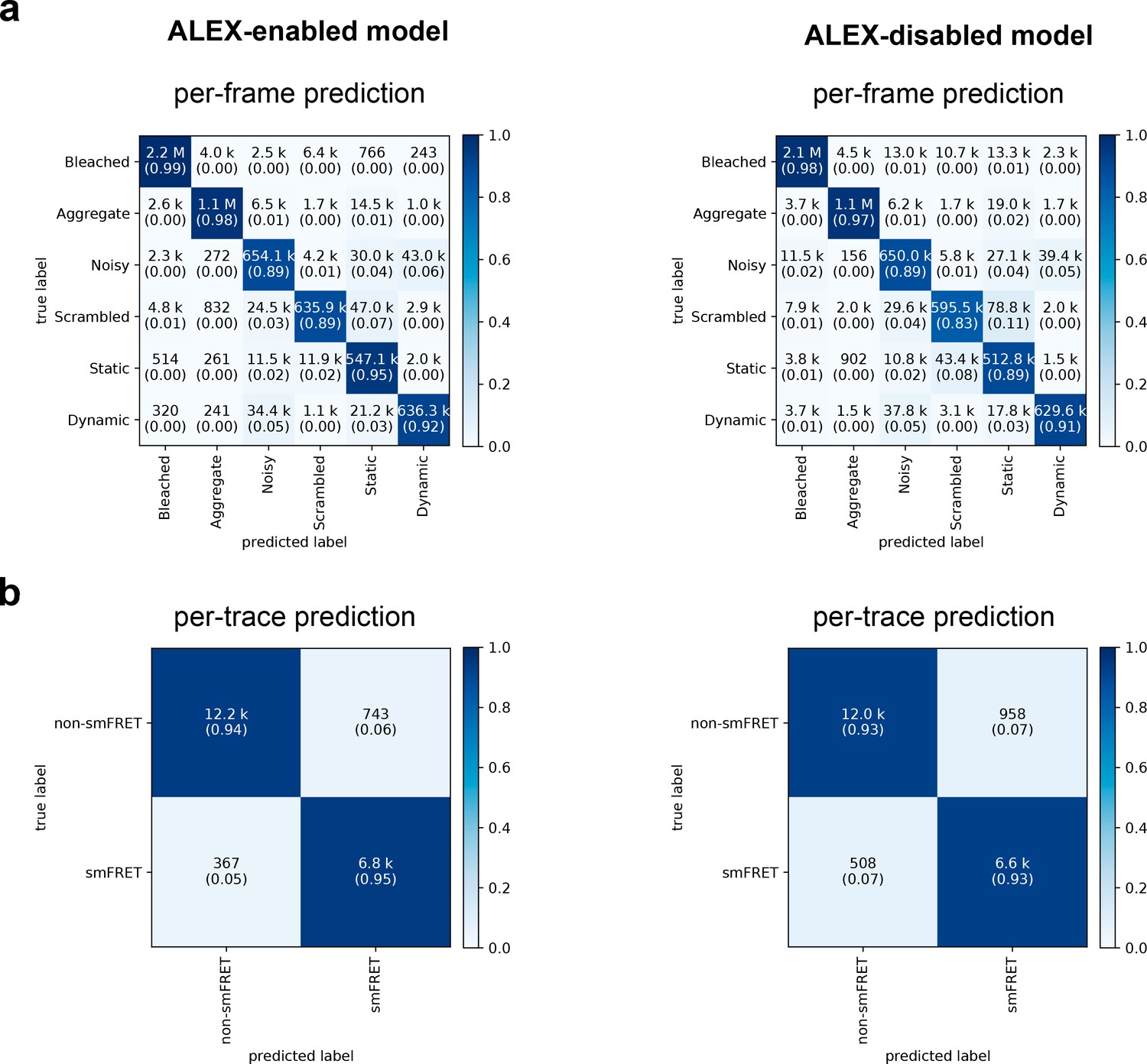
Confusion matrices of DeepFRET classification based on the ground truth data test.
(a) Classification accuracy of data in the six categories for the ALEX-enabled model, or the ALEX-disabled model. The absolute number of frames is shown while the fractions for each classification is displayed in parentheses (as calculated row-wise for each true label). The diagonal percentages show the accurate classification of DeepFRET (b) per-trace classification accuracy based on accepting only traces that are classified as smFRET (static/dynamic), and non-FRET data.
Figure 3—figure supplement 1
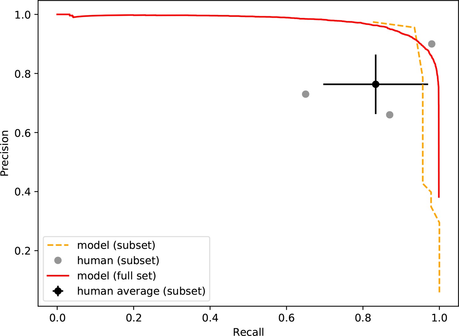
Precision-recall of the neural network and human participants.
Precision is plotted against recall for all precision on a simulated dataset containing 46 true smFRET traces and 954 non-smFRET traces. Additionally, the precision-recall for the entire test set (20,000 traces) is plotted for the model. The error bars on the average participant performance represent the standard deviation of the three individual participants.
-
Figure 3—figure supplement 1—source data 1
Data underlying Figure 3—figure supplement 1.
- https://cdn.elifesciences.org/articles/60404/elife-60404-fig3-figsupp1-data1-v1.zip
Figure 4 with 4 supplements

Method evaluation on real previously published smFRET data.
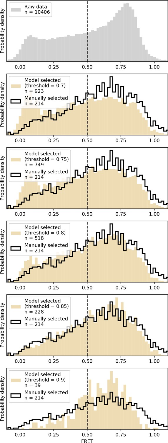
(a) Raw FRET distribution as it would look before any sorting to remove incomplete or multi-labeled proteins, aggregates, cross talk, etc. (b, c) Comparison of DeepFRET data selection with published distributions for 0.7 in (b) and 0.85 in (c) thresholds. At the DeepFRET score threshold of 0.85, a high-fidelity data selection is achieved resulting in a similar distribution as compared to manual selection.
-
Figure 4—source data 1
Data underlying Figure 4 and Figure 4—figure supplements 2–4.
- https://cdn.elifesciences.org/articles/60404/elife-60404-fig4-data1-v1.zip
Figure 4—figure supplement 1
DeepFRET applied to experimentally-obtained data.
We applied DeepFRET to a previously obtained smFRET dataset on CRISPR-Cas12a. At the DeepFRET threshold of ~0.8–0.85 an excellent agreement with previously used sorting methodologies involving manual inspection of data was achieved.
Figure 4—figure supplement 2
Distribution of trace quality of the experimental dataset.
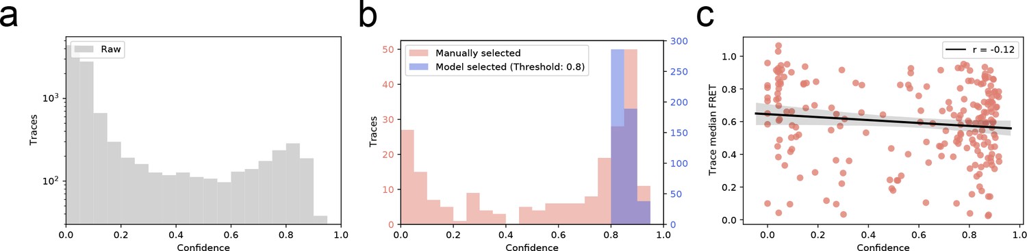
(a) The predicted confidence score of every trace in experimentally recorded dataset (b) Confidence score distribution of manual versus automatic selection of smFRET traces. Automatic selection exclusively accepts high-confidence traces. (c) Pearson’s test displaying no correlation (r = −0.12) between predicted trace confidence and mean FRET in the manually selected dataset.
Figure 4—figure supplement 3

Comparison of DeepFRET, SPARTAN, iSMS, HAMMY, and ebFRET performance on simulated, ground truth data.
(a) 200 simulated, ground truth smFRET traces (left) were merged with 1800 simulated, non-smFRET traces (middle) to yield a combined distribution of 2000 traces (right). (b) Performance of DeepFRET, SPARTAN, iSMS, HAMMY, and ebFRET on the simulated data employing various sorting criteria. In SPARTAN, six commonly used thresholds were employed on parameters including donor/acceptor correlation, SNR, intensity, FRET lifetime, exclusion of photoblinking, and step-wise drops in fluorescence intensity. In iSMS, aggregates were removed by intensity thresholds with subsequent sorting based on stoichiometries of ~0.4–0.6 and removal of FRET outliers. In HAMMY, sorting was based on intensity thresholds, while in ebFRET, sorting was based on the removal of FRET outliers (0 < E < 1). Data is displayed without applying correction factors. Note that, expert users can navigate through all thresholds and define their own to further, and even more accurately, optimize data selection of both SPARTAN and iSMS, while HAMMY and ebFRET may require additional manual selection or sorting via other software packages. DeepFRET only required a single quality threshold of 0.8.
Figure 4—figure supplement 4
Comparison of DeepFRET, SPARTAN, and iSMS performance on the published experimental data.
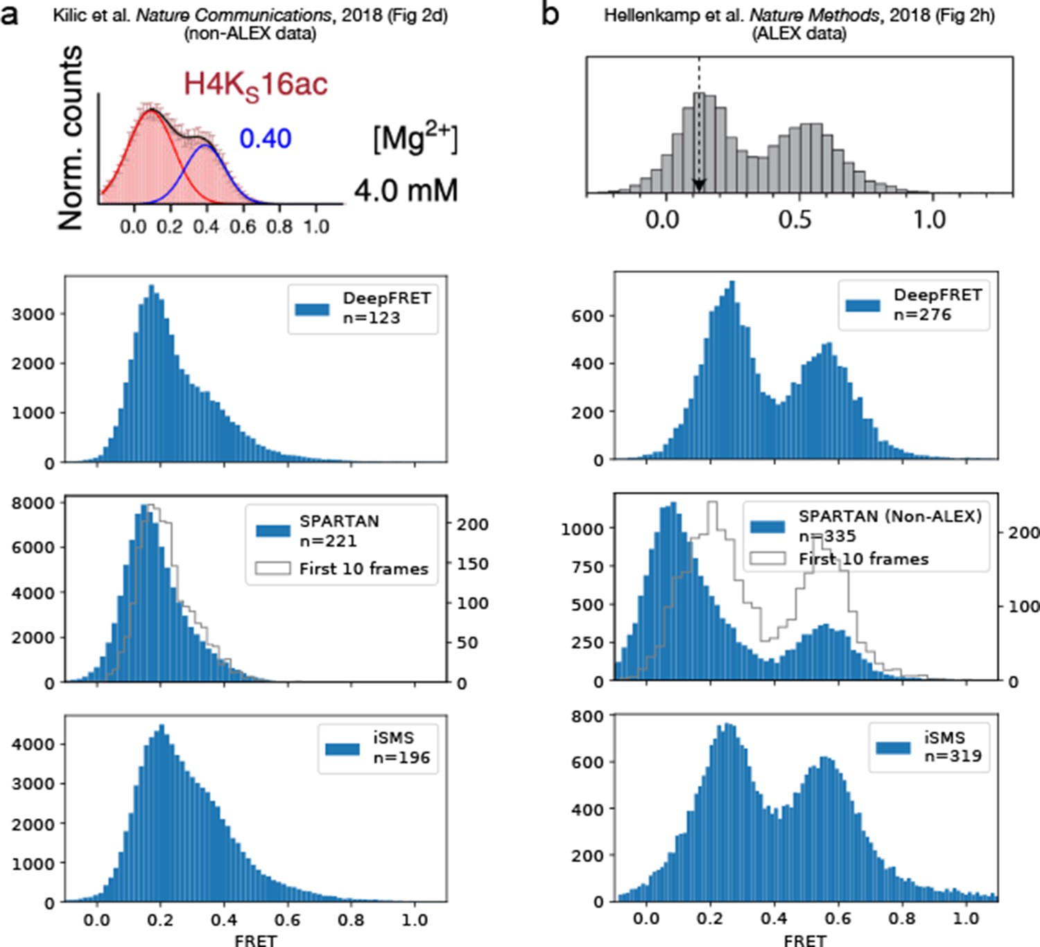
DeepFRET, SPARTAN, and iSMS performance on (a) non-ALEX data published by Kilic et al., 2018 and (b) ALEX data published by Hellenkamp et al., 2018. In both cases, all software packages were found to reproduce the published FRET distributions from raw tif files with a little discrepancy. The raw movies resulted in 294 and 719 traces, respectively, before sorting. Data selection relied on removing aggregates and using stoichiometries of ~0.4–0.6 for iSMS and the commonly used thresholds for SPARTAN including thresholds on donor/acceptor correlation, SNR, intensity, FRET lifetime, exclusion of photoblinking step-wise drops in fluorescence intensity, and using 10 first frames minimizing bleaching effect. Note that expert users can navigate through all thresholds and define their own to further, and even more accurately, optimize data selection of iSMS and SPARTAN. In DeepFRET, a single quality score was used to sort traces. Data selection resulted in removal of ~40–60% of the traces in all cases, and are displayed without applying correction factors.
Additional files
Download links
A two-part list of links to download the article, or parts of the article, in various formats.
Downloads (link to download the article as PDF)
Open citations (links to open the citations from this article in various online reference manager services)
Cite this article (links to download the citations from this article in formats compatible with various reference manager tools)
DeepFRET, a software for rapid and automated single-molecule FRET data classification using deep learning
eLife 9:e60404.
https://doi.org/10.7554/eLife.60404


