Research Article

Computational modeling of threat learning reveals links with anxiety and neuroanatomy in humans

Emotion and Development Branch, National Institute of Mental Health, National Institutes of Health, United States
Laboratory of Neuropsychology, National Institute of Mental Health, National Institutes of Health, United States
Department of Psychiatry and Human Behavior, Brown University Warren Alpert Medical School, United States
Department of Psychology, University of Miami, United States
Department of Psychology, University of California, Riverside, United States
Psychology Department, University of Haifa, Israel

Apr 27, 2022

https://doi.org/10.7554/eLife.66169

Open access
Copyright information

Figures
Tables
Additional files

9 figures, 4 tables and 3 additional files

Figures

Figure 1 with 1 supplement

Download asset Open asset

Threat learning task and physiological data.

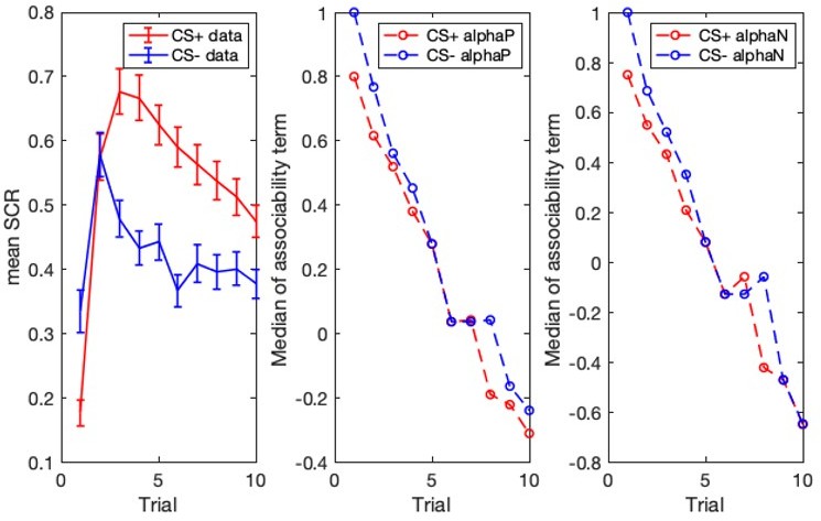
Top: Schematic representation of the threat learning paradigm. During the pre-conditioning phase, the designated threat (CS+) and safety (CS-) stimuli were presented without reinforcement. During the conditioning phase, the CS + was paired with a fearful face co-terminating with a scream (UCS); the CS- was never reinforced. During the extinction phase, both CS + and CS- were not reinforced by the UCS. Bottom: Mean raw skin conductance response for the CS + and CS- by task phase and trial. *Note:* Trial number indicates the nth trial for that stimulus. However, the CS+ and CS- trials were presented in counterbalanced order throughout the task. CS = conditioned stimulus; UCS = unconditioned stimulus. Error bars indicate one standard error of the mean.

Figure 1—figure supplement 1

Download asset Open asset

Histogram depicting the distribution of the standardized anxiety severity scores across the sample.

Figure 2 with 3 supplements

Download asset Open asset

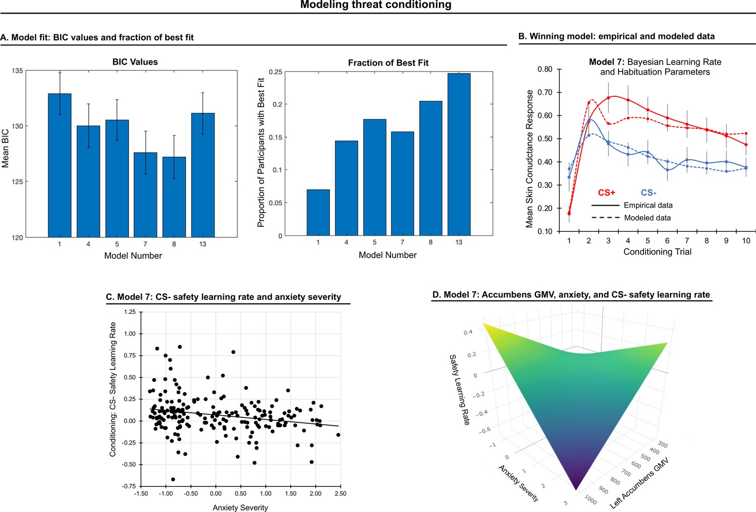
Modeling threat conditioning.

(A) Bars in left panel depict BIC values for each of the fourteen models fit to the CS- and CS + conditioning data. Error bars indicate one standard error of the mean. Bars in right panel depict the proportion of participants for whom each model provided the best fit. (B) Based on model fit indices, model 7 was chosen as the best-fitting model for conditioning data. Graphs depict empirical skin conductance data (full line) and fitted data (dashed line) for model 7 fitted to CS+ (red) and CS- (blue) conditioning data. Data are smoothed for display purposes only. (C) Association between model 7’s CS- learning rate parameter and anxiety severity. (D) The association between model 7’s CS- learning rate parameter and anxiety severity was moderated by left accumbens gray matter volume (GMV).

Figure 2—figure supplement 1

Download asset Open asset

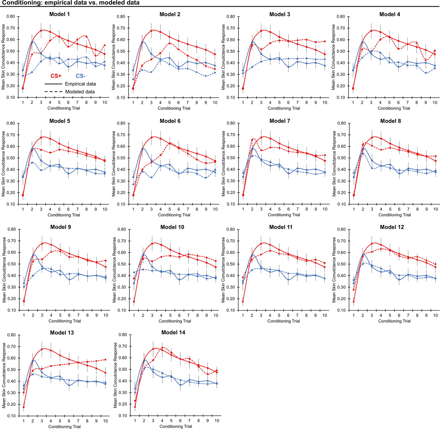
Threat conditioning model fits.

Graphs depict empirical skin conductance data (full line) and fitted data (dashed line) for each of the models fitted to CS+ (red) and CS- (blue) conditioning data. Data are smoothed for display purposes only.

Figure 2—figure supplement 2

Download asset Open asset

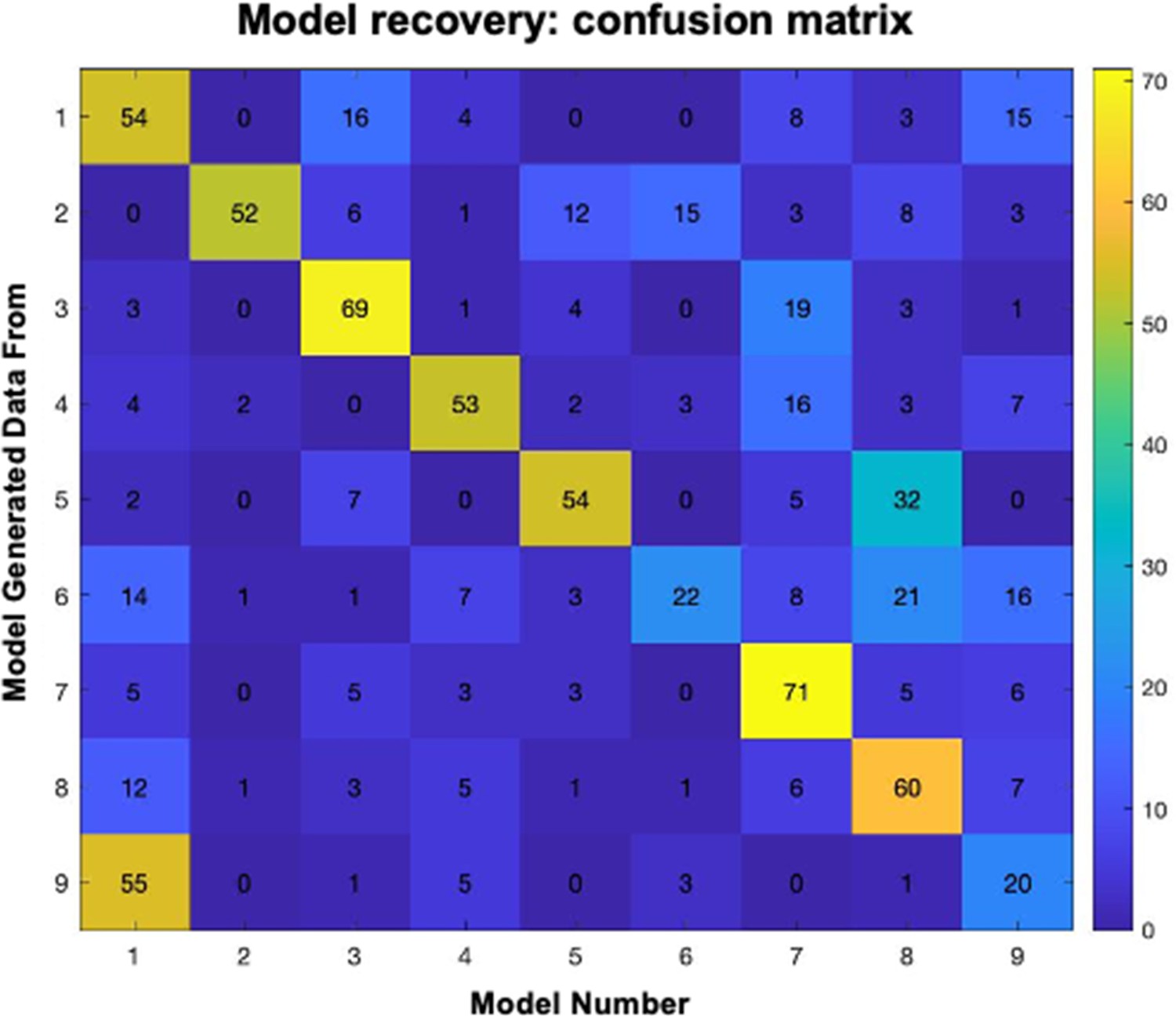
Conditioning model recovery.

Confusion matrix depicting distribution of selected models when data were simulated with each model. For each row (model), columns depict the number of simulated datasets that were identified as generated from that model.

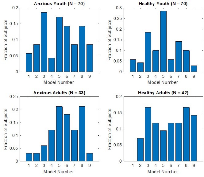
Figure 2—figure supplement 3

Download asset Open asset

Proportions of participants for whom each model provided the best fit, when the sample is divided into anxiety (patients vs healthy comparisons) and age (youth vs adults) groups.

Figure 3 with 1 supplement

Download asset Open asset

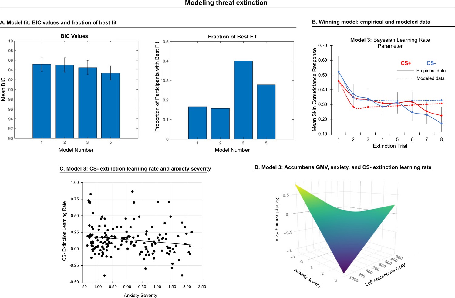
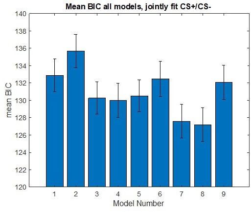
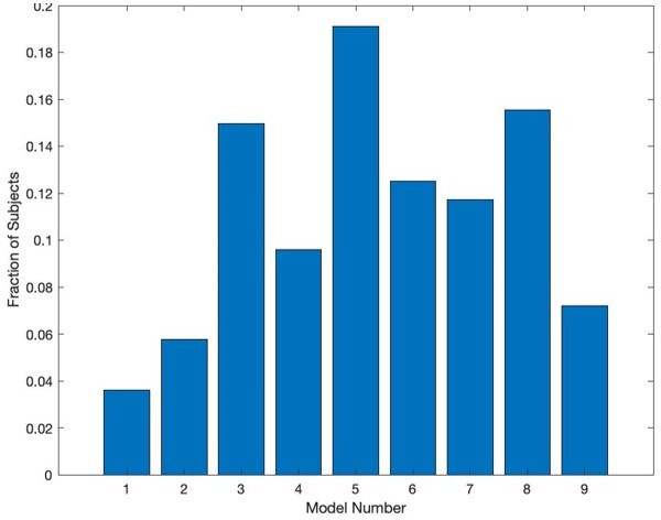
Modeling threat extinction.

(A) Bars in left panel depict BIC values for each of the twelve models fit to the CS- and CS+ extinction data. Error bars indicate one standard error of the mean. Bars in right panel depict the proportion of participants for whom each model provided the best fit. (B) Based on model fit indices, model 3 was chosen as the best-fitting model for extinction data. Graphs depict empirical skin conductance data (full line) and fitted data (dashed line) for model 3 fitted to CS+ (red) and CS- (blue) extinction data. Data are smoothed for display purposes only. (C) Association between model 3’s CS- extinction rate parameter and anxiety severity; this association is only trend-level significant. (D) The association between model 3’s CS- learning rate parameter and anxiety severity was moderated by left accumbens gray matter volume (GMV); this association is only trend-level significant.

Figure 3—figure supplement 1

Download asset Open asset

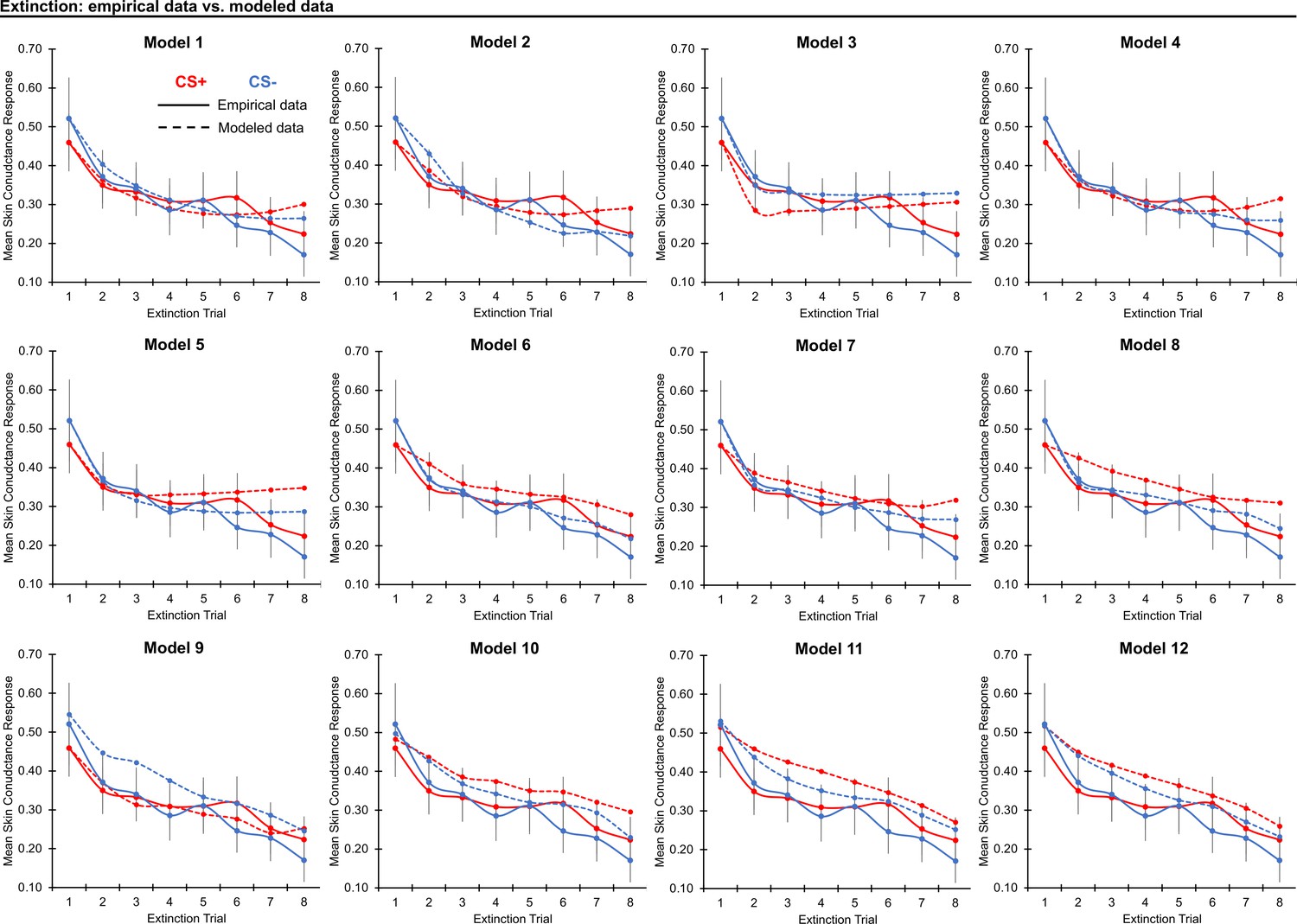
Threat extinction model fit.

Graphs depict empirical skin conductance data (full line) and fitted data (dashed line) for each of the models fitted to CS+ (red) and CS- (blue) extinction data. Data are smoothed for display purposes only.

Author response image 1

Download asset Open asset

Author response image 2

Download asset Open asset

Author response image 3

Download asset Open asset

Author response image 4

Download asset Open asset

Author response image 5

Download asset Open asset

Author response image 6

Download asset Open asset

Model fit: BIC values and fraction of best fit.

Tables

Table 1

Specifications and estimated free parameters for each model fit to the CS- and CS+.

Model	Model specification	Free parameters	Initialization values
1.RW	$ν_{C S} (t + 1) = ν_{C S} (t) + α δ$	$α_{C S +}, α_{C S -}$ ,	$ν_{C S +} (0) = V_{i}$ $ν_{C S -} (0) = V_{i}$ where v_i is the SCR value from the last habituation trial (acquisition) and SCR value from the first extinction trial (extinction)
2.RW with inertia	$ν_{C S} (t + 1) = ν_{C S} (t) + α (t) δ^{i n}$ , whereby, $δ^{i n} (t) = \sum_{k = 0}^{k_{m}} δ (t - k)$ , with m=number of recent trials	$α_{C S +}, α_{C S -}$	same as model 1
3.RW with Bayesian learning-rate decay	$ν_{C S} (t + 1) = ν_{C S} (t) + α (t) δ$ , with $α (t) = \frac{α}{s q r t (t)}$	$α_{C S +}, α_{C S -}$	same as model 1
4.RW with habituation	$v_{C S} (t + 1) = v_{C S} (t) + α δ$ , with $ν_{C S} (t)$ multiplied by $e^{- φ_{C S} [t - t_{0}]^{+}}$ after update	$α_{C S +}, α_{C S -}; φ_{C S +}, φ_{C S -}$	same as model 1
5.RW with inertia and Bayesian learning-rate decay	$v_{C S} (t + 1) = v_{C S} (t) + α (t) δ^{i n}$ , with $α (t) = \frac{α}{s q r t (t)}$ , and $δ^{i n} (t) = \sum_{k = 0}^{k_{m}} δ (t - k)$ , with m=number of recent trials	$α_{C S +}, α_{C S -}$	same as model 1
6.RW with inertia and habituation	$ν_{C S} (t + 1) = ν_{C S} (t) + α (t) δ^{i n}$ , whereby $δ^{i n} (t) = \sum_{k = 0}^{k_{m}} δ (t - k)$ , with m=number of recent trials, and $ν_{C S} (t)$ multiplied by $e^{- φ_{C S} [t - t_{0}]^{+}}$ after update	$α_{C S +}, α_{C S -}; φ_{C S +}, φ_{C S -}$	same as model 1
7.RW with Bayesian learning-rate decay and habituation	$ν_{C S} (t + 1) = ν_{C S} (t) + α δ$ , whereby $α (t) = \frac{α}{s q r t (t)}$ and $v_{C S} (t)$ multiplied by $e^{- φ [t - t_{0}]^{+}}$ after update		same as model 1
8.RW with inertia and Bayesian learning-rate decay, and habituation	$ν_{C S} (t + 1) = ν_{C S} (t) + α (t) δ^{i n}$ , whereby, $α (t) = \frac{α}{s q r t (t)}$ and $δ^{i n} (t) = \sum_{k = 0}^{k_{m}} δ (t - k)$ , with m=number of recent trials, and $ν_{C S} (t)$ multiplied by $e^{- φ_{C S} [t - t_{0}]^{+}}$ after update	$α_{C S} +, α_{C S} -; φ_{C S} +, φ_{C S} -$	same as model 1
9.RW-PH hybrid	$ν_{C S} (t + 1) = ν_{C S} (t) + κ α δ$ , whereby	$γ_{C S +}, γ_{C S -}, κ_{C S +}, κ_{C S -}$	$α_{C S +} (0) = 1$ $α_{C S -} (0) = 1$
10.Hybrid(V) Li et al., 2011	(Changing V_n for $ν_{C S} (t + 1) δ (n) = b U C S (n) - V_{n} (x_{n})$ ), where bUCS(n)=1 if a UCS was delivered and bUCS(n)=0 if no UCS was delivered (b indicates binary UCS). SCR was then predicted using a regression: $p S C R (V)_{n} \sim N (β_{0} + β_{1} V_{n} (x_{n}), σ)$ The squared error: $H y b r i d (V) E r r o r = (p S C R (V) - S C R)^{2}$	$γ_{C S +}, γ_{C S -}, κ_{C S +}, κ_{C S -}, β_{0}, β_{1}$	$\begin{array}{ll} α_{C S} + (0) = 1 \\ α_{C S} - (0) = 1 \\ v_{C S} + (0) = v_{i} \\ v_{C S} - (0) = v_{i} \end{array}$ where v_i is the SCR value on the last habituation trial and SCR value from the first extinction trial (extinction)
11.Hybrid(α) Li et al., 2011	Same as model 10 (changing V_n for $ν_{C S} (t + 1)$ ) except $p S C R (α_{n}) \sim N (β_{0} + β_{1} α_{n} (x_{n}), σ)$ The squared error: $H y b r i d (α) E r r o r = (p S C R (α) - S C R)^{2}$	$γ_{C S +}, γ_{C S -}, κ_{C S +}, κ_{C S -}, β_{0}, β_{1}$	same as model 10
12.Hybrid (V+α) Li et al., 2011	Same as model 10 changing V_n for $ν_{C S} (t + 1)$ with additional regression such that: $p S C R (V, α) n \sim N (β 0 + β 1 V n (x n) + β 2 α n (x n), σ)$ $H y b r i d (V + α) E r r o r = (p S C R (V, α) - S C R)^{2}$	$γ_{C S +}, γ_{C S -}, κ_{C S +}, κ_{C S -}, β_{0}, β_{1}$	same as model 10
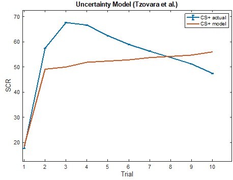
13.Mixed prior mean and uncertainty model Tzovara et al., 2018	$h_{C S} (t) = - l n (α_{C S} + β_{C S})$ $z_{C S} (t) = h_{C S} (t) + E [θ]$ Where $B (α_{C S}, β_{C S})$ is a Beta function whose parameters are updated according to: $α_{C S} (t) = α_{C S} (t - 1) + u (t - 1)$ $β_{C S} (t) = β_{C S} (t - 1) - u (t - 1) + 1$ Where $u (t) = 1$ if a US occurred and $u (t) = 0$ otherwise. $β_{0}, β_{1}$ are the regression parameters relating $z_{C S} (t)$ to SCR	$β_{0}, β_{1}$	$α_{C S} (0) = 1 β_{C S} (0) = 1$
14.Mixed prior mean and uncertainty model (Model 13) Tzovara et al., 2018 with habituation	Same as model 13 with the addition: $h_{C S} (t)$ multiplied by $e^{- φ_{C S} [t - t_{0}]^{+}}$ after update for habituation	$β_{0}, β_{1}, φ_{C S +}, φ_{C S -}$	same as model 13

Appendix 1—table 1

Demographics (sex, age, IQ) and anxiety severity (by diagnosis: anxious/healthy; by continuous anxiety scores on the Screen for Child Anxiety Related Emotional Disorders or ) for participants who were included or excluded from data analysis due to excessive missing data.

Differences between included and excluded participants were tested using chi-squared or independent-samples t-tests.

	Excluded	Included	Test Statistic
N	136 (94 F)	215 (116 F)
% Female	69.11	53.95	$χ_{(1)}^{2}$ = 7.35, P=.006
N Anxiety diagnosis	55	104	$χ_{(1)}^{2}$ = 1.81, P=.18
N Healthy	85	111	$χ_{(1)}^{2}$ = 3.56, P=.06
Mean (SD) age	23.40 (9.16)	18.76 (9.39)	t(302.29) = 4.62, P<.001
Mean (SD) anxiety	–0.09 (0.89)	0.05 (1.06)	t(288.66) = 1.27, P=.21
Mean (SD) IQ	114.68 (13.32)	113.98 (11.90)	t(271) = .50, P=.61

Appendix 1—table 2

Corelations between the actual parameters and recovered parameters for each of the 14 models for acquisition data.

Models in bold met the criteria for model comparison (all corelation values for all parameters >0.20). Note that the last row reflects an additional variant of the Tzovara et al. model with two additional habituation parameters (habituation for CS+ and CS- for 6 total parameters) that was examined for completeness (see Methods).

Model	Parameter 1, CS+ learning Rate	Parameter 2, CS- learning Rate	Parameter 3, CS+ habituation	Parameter 4, CS- habituation
1	0.99	0.56
2 (inertia)	0.86	0.22
3 (Bayesian)	0.52	0.21
4	0.76	0.99	>0.99	0.99
5 (inertia +Bayesian)	0.74	0.46
6 (inertia)	0.38	0.17	0.53	>0.99
7 (Bayesian)	0.59	0.42	0.98	>0.99
8 (inertia +Bayesian)	0.52	0.62	0.96	>0.99
	Parameter 1, CS +learning Rate	Parameter 2, CS- learning Rate	Parameter 3, CS +learning rate update	Parameter 4, CS- learning rate update	Parameter 5, regression β_o	Parameter 6 regression β₁	Parameter 7 regression β₂
9	0.53	0.13	0.52	0.02
10	–0.09	0.04	–0.37	0.46	0.35	0.21
11	0.49	0.07	–0.37	0.46	0.35	0.21
12	0.34	0.04	–0.39	0.66	0.002	0.02	0.99
	Parameter 1, β_o	Parameter 2, β₁	Parameter 5, CS+ habituation	Parameter 4, CS- habituation
13	0.90	0.96
14	0.81	0.90	–0.03	0.33

Appendix 1—table 3

Correlations between the actual parameters and recovered parameters for each model for extinction data.

Models in bold met the criteria for model comparison (all correlation values for all parameters > 0.20).

Model	Parameter 1, CS+ learning rate	Parameter 2, CS- learning rate	Parameter 3, CS+ habituation	Parameter 4, CS- habituation
1	0.59	0.45
2 (inertia)	0.51	0.46
3 (Bayesian)	0.83	0.69
4	0.28	0.07	0.46	0.93
5 (inertia + Bayesian)	0.80	0.82
6 (inertia)	0.49	0.27	0.05	-0.04
7 (Bayesian)	0.32	0.40	0.05	0.40
8 (inertia + Bayesian)	0.22	0.25	-0.003	0.01
	Parameter 1, CS+ learning rate	Parameter 2, CS- learning rate	Parameter 3, CS+ learning rate update	Parameter 4, CS- learning rate update	Parameter 5, regression β_o	Parameter 6, regression β₁	Parameter 7, regression β₂
9	0.47	0.33	0.11	0.01
10	0.28	0.01	0.01	0.03	0.82	0.19
11	0.85	0.11	0.99	0.86	–0.31	–0.03
12	0.99	-0.002	0.99	0.93	0.90	0.90	–0.01

Additional files

Transparent reporting form: https://cdn.elifesciences.org/articles/66169/elife-66169-transrepform1-v2.docx
Download elife-66169-transrepform1-v2.docx
Source code 1 Code for reinforcement learning models.: https://cdn.elifesciences.org/articles/66169/elife-66169-code1-v2.zip
Download elife-66169-code1-v2.zip
Source code 2 Code for imaging processing and analysis.: https://cdn.elifesciences.org/articles/66169/elife-66169-code2-v2.zip
Download elife-66169-code2-v2.zip

Download links

A two-part list of links to download the article, or parts of the article, in various formats.

Downloads (link to download the article as PDF)

Open citations (links to open the citations from this article in various online reference manager services)

Mendeley

Cite this article (links to download the citations from this article in formats compatible with various reference manager tools)

Rany Abend
Diana Burk
Sonia G Ruiz
Andrea L Gold
Julia L Napoli
Jennifer C Britton
Kalina J Michalska
Tomer Shechner
Anderson M Winkler
Ellen Leibenluft
Daniel S Pine
Bruno B Averbeck

(2022)

Computational modeling of threat learning reveals links with anxiety and neuroanatomy in humans

eLife 11:e66169.

https://doi.org/10.7554/eLife.66169

Share this article

Cite this article

Threat learning task and physiological data.

Histogram depicting the distribution of the standardized anxiety severity scores across the sample.

Modeling threat conditioning.

Threat conditioning model fits.

Conditioning model recovery.

Proportions of participants for whom each model provided the best fit, when the sample is divided into anxiety (patients vs healthy comparisons) and age (youth vs adults) groups.

Modeling threat extinction.

Threat extinction model fit.

Model fit: BIC values and fraction of best fit.

Specifications and estimated free parameters for each model fit to the CS- and CS+.

Demographics (sex, age, IQ) and anxiety severity (by diagnosis: anxious/healthy; by continuous anxiety scores on the Screen for Child Anxiety Related Emotional Disorders or ) for participants who were included or excluded from data analysis due to excessive missing data.

Corelations between the actual parameters and recovered parameters for each of the 14 models for acquisition data.

Correlations between the actual parameters and recovered parameters for each model for extinction data.

Transparent reporting form

Source code 1

Source code 2

Downloads (link to download the article as PDF)

Open citations (links to open the citations from this article in various online reference manager services)

Cite this article (links to download the citations from this article in formats compatible with various reference manager tools)