Force propagation between epithelial cells depends on active coupling and mechano-structural polarization
- Université Grenoble Alpes, CNRS, LIPhy, France
- Institute for Theoretical Physics, Heidelberg University, Germany
- BioQuant–Center for Quantitative Biology, Heidelberg University, Germany
- London Centre for Nanotechnology, University College London, United Kingdom
- Department of Cell and Developmental Biology, University College London, United Kingdom
- Institute for the Physics of Living Systems, University College London, United Kingdom
Figures
Figure 1 with 1 supplement
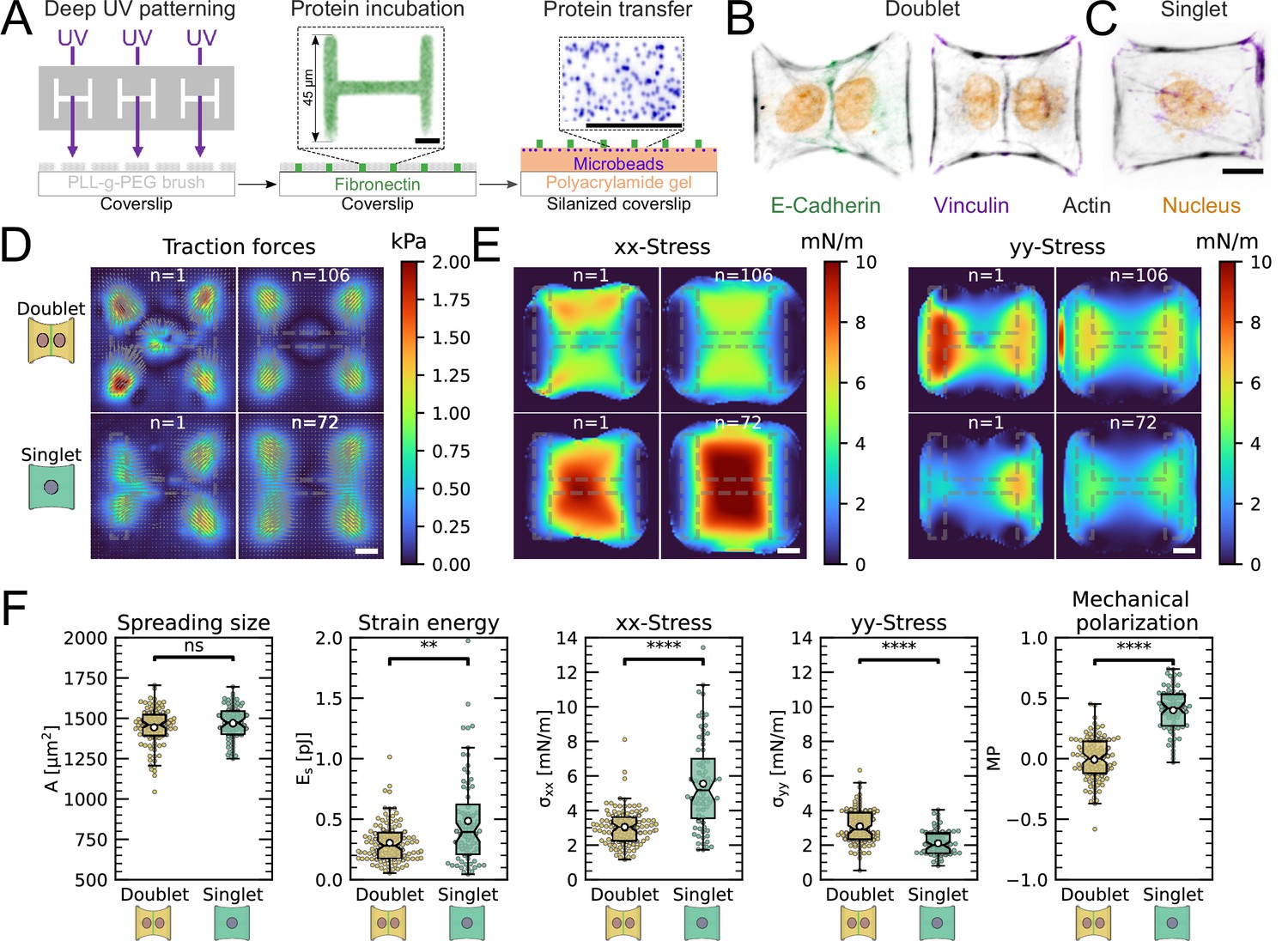
The cell–cell junction leads to a decrease in mechanical polarization.
(A) Cartoon of the micropatterning process on soft substrates, allowing to control cell shape and measure forces at the same time by embedding fluorescent microbeads into the gel and measuring their displacement. The middle panel shows the used pattern geometry, an H with dimensions of × . (B, C) Immunostaining of opto-MDCK cells plated on H-patterns and incubated for before fixing. Actin is shown in black, E-cadherin in green, vinculin in violet, and the nucleus in orange. (B) The left and right images show a representative example of a doublet. (C) A representative example of a singlet. (D) Traction stress and force maps of doublets (top) and singlets (bottom) with a representative example on the left and an average on the right. (E) Cell stress maps calculated by applying a monolayer stress microscopy algorithm to the traction stress maps, with a representative example on the left and an average on the right. (F) From left to right, boxplots of spreading size, measured within the boundary defined by the stress fibers. Strain energy, calculated by summing up the squared scalar product of traction force and displacement field divided by two xx-stress and yy-stress calculated by averaging the stress maps obtained with monolayer stress microscopy. Degree of polarization, defined as the difference of the average xx- and yy-stress normalized by their sum. Doublets are shown in yellow and singlets are shown in green. The figure shows data from n = 106 doublets from N = 10 samples and n = 72 singlets from N = 12 samples. All scale bars are long.
Figure 1—figure supplement 1

Immunostaining of opto-MDCK cells plated on H-patterns and incubated for before fixing.
Actin, E-cadherin, vinculin, and the nucleus are shown. The top and middle rows show a representative example of a doublet, and the bottom row shows a representative example of a singlet. Scale bar is long.
Figure 2
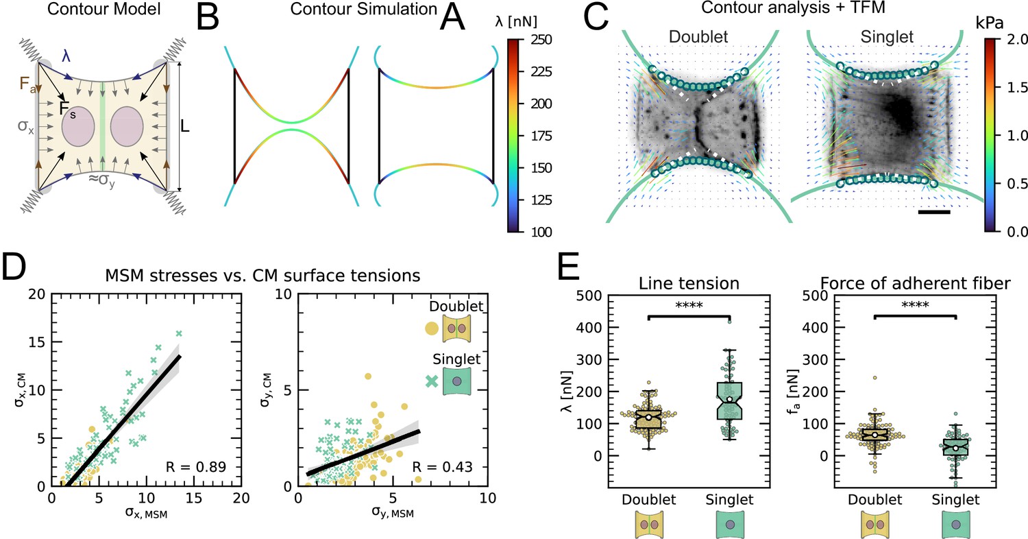
The cell–cell junction leads to a redistribution of tension from free to adherent peripheral stress fiber.
(A) Cartoon of the contour model used to analyze the shape of the doublets and singlets. (B) Finite element method (FEM) simulation of the contour with left and right. (C) Actin images of doublets (left) and singlets (right) with traction stresses (arrows), tracking of the free fiber (blue circles), elliptical contour fitted to the fiber tracks (green line), and tangents to the contour at adhesion point (white dashed line). The scale bar is long. (D) Correlation plot of monolayer stress microscopy (MSM) stresses and CM surface tensions. MSM stresses were calculated by averaging the stress maps obtained with monolayer stress microscopy, and the surface tensions were obtained by the contour model analysis, where was measured on the traction force microscopy (TFM) maps by summing up the x-traction stresses in a window around the center of the vertical fiber and was determined by fitting the resulting ellipse to the tracking data of the free fiber. Doublets are shown as yellow dots, and singlets are shown as green crosses. The black line shows the linear regression of the data, and the shaded area shows the 95% confidence interval for this regression. The R-value shown corresponds to the Pearson correlation coefficient. (E) Boxplots of line tension (left) and force of adherent fiber (right) as defined in panel (A). Both values were calculated by first calculating the force in each corner by summing up all forces in a radius of around the peak value and then projecting the resulting force onto the tangent of the contour for the line tension and onto the y-axis for the force of adherent fiber. Doublets are shown in yellow, and singlets are shown in green. The figure shows data from n = 106 doublets from N = 10 samples and n = 72 singlets from N = 12 samples. All scale bars are long.
Figure 3 with 5 supplements
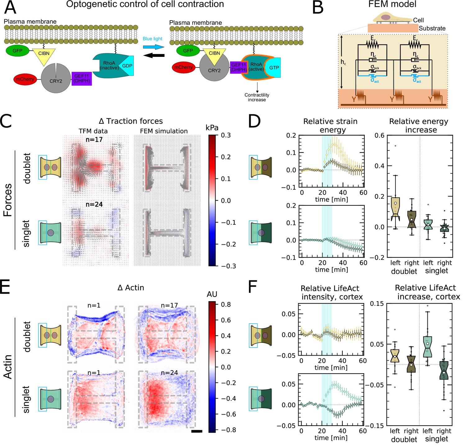
Local activation of RhoA leads to stable force increase in both the activated and the nonactivated cell in doublets, but destabilizes force homeostasis in singlets.
(A) Cartoon of the optogenetic CIBN/CRY2 construction used to locally activate RhoA. (B) Cartoon of the FEM continuum model used to explain optogenetic experiments. (C) Difference of average traction force maps after and before photoactivation of cell doublets (top) and singlets (bottom). Maps on the left show the traction force microscopy (TFM) data, and maps on the right show the result of the FEM simulations with an active response of the right cell. (D) Relative strain energies of doublets (top) and singlets (bottom) with local photoactivation, divided into left half (bright) and right half (dark). One frame per minute was acquired for 60 min, and cells were photoactivated with one pulse per minute for 10 min between minute 20 and minute 30. Strain energy curves were normalized by first subtracting the individual baseline energies (average of the first 20 min) and then dividing by the average baseline energy of all cell doublets/singlets in the corresponding datasets. Data is shown as circles with the mean ± SEM. Boxplots on the right show the value of the relative strain energy curves 2 min after photoactivation, that is, at minute 32. (E) Difference of actin images after and before photoactivation of doublets (top) and singlets (bottom), with an example on the left and the average on the bottom. All scale bars are long. (F) LifeAct intensity measurement inside the cells over time (left) of left half (bright) vs. right half (dark) of doublets (top) and singlets (bottom) after local photoactivation. Boxplots on the right show the relative actin intensity value after 2 min after photoactivation of activated vs. nonactivated half. The figure shows data from n = 17 doublets from N = 2 samples and n = 17 singlets from N = 6 samples. All scale bars are long.
Figure 3—figure supplement 1

LifeAct images of doublets and singlets on H-patterns, quantification of mechano-structural polarization and measurement of LifeAct intensities of stress fibers in response to optogenetical activation of RhoA.
(A) LifeAct images of some example opto-MDCK doublets (left) and singlets (right) plated on H-patterns. (B) Correlation plot of mechanical and structural polarization. The black line shows the linear regression of the data, and the shaded area shows the 95% confidence interval for this regression. The R-value shown corresponds to the Pearson correlation coefficient. Scale bar is long. (C) LifeAct intensity measurement on periphery of cells over time (left) of left half (bright) vs. right half (dark) of doublets (top) and singlets (bottom) after local photoactivation. Boxplots on the right show the relative actin intensity value after 2 min after photoactivation of activated vs. nonactivated half.
Figure 3—figure supplement 2
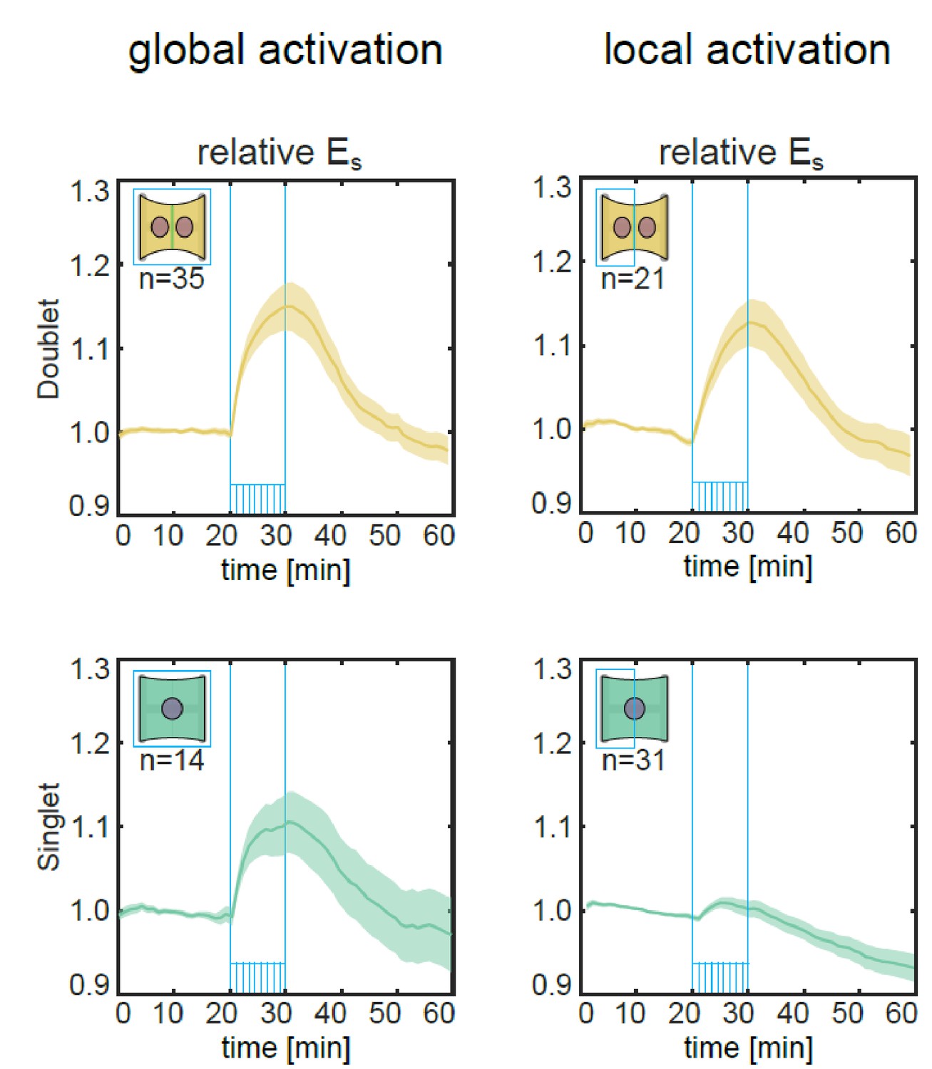
Relative strain energies of local (left) vs. global (right) photoactivation of doublets (top) and singlets (bottom).
Figure 3—figure supplement 3
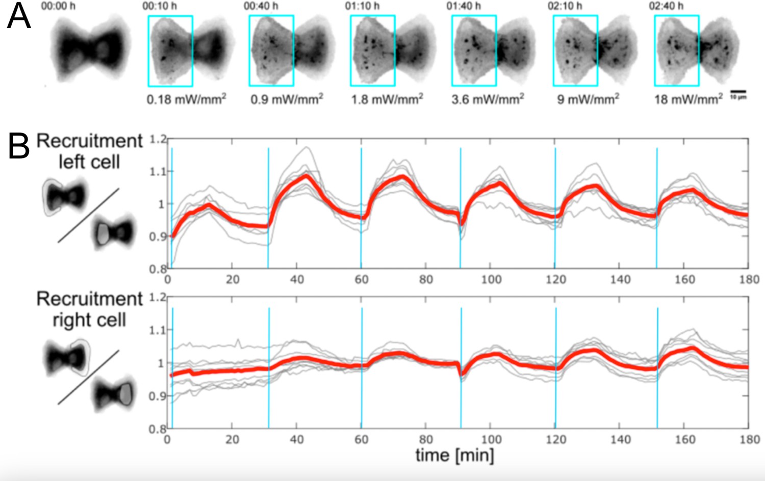
Recruitment of CRY2 to the membrane in left vs. right cell in response to optogenetic activation with varying light intensities.
(A) Fluorescence images of CRY2 in MDCK cell doublets in response to photoactivation pulse of increasing power. (B) CRY2 recruitment from the cytosol to the plasma membrane, quantified by measuring the ratio of intensities in the lamellipodium vs. the cytosol.
Figure 3—figure supplement 4
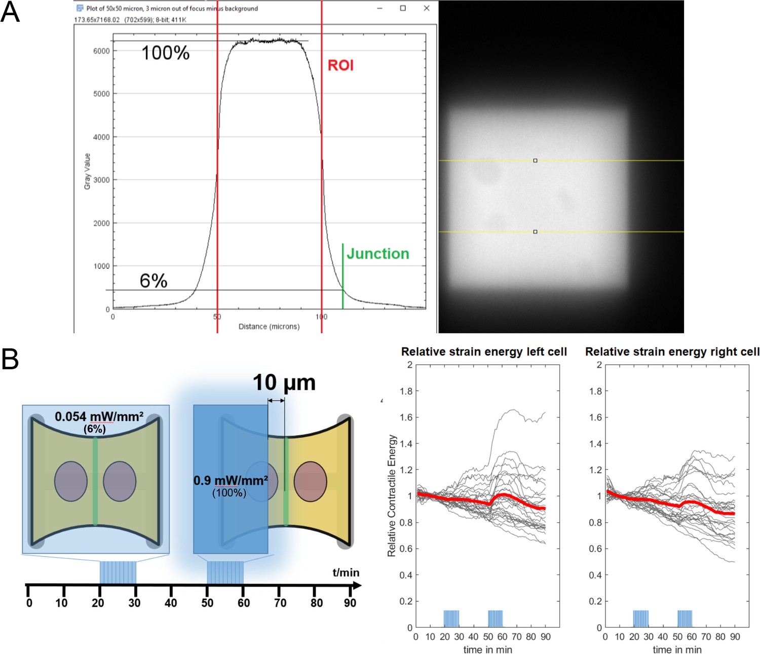
Strain energy increase of non-activated cell is not caused by accidental photoactivation through stray light.
(A) Fluorescence image of a homogeneously coated coverslip, illuminated on a rectangular zone with a digitial micromirror device (DMD) and the horizontal intensity profile. The background was subtracted from the image before making the measurements. The peak intensity drops to 6% over a distance of , so all local activation routines were placed away from the junction. (B) Left: a cartoon describing the experiment. First, the whole doublet is activated at low light intensity () and then only the left cell is activated with higher intensity (). The intensity of the first activation routine corresponds to the intensity right at the junction from the second activation routine. Right: curves show the strain energy stored in the substrate under the left cell (left) and under the right cell (right). The strain energy curves were normalized by the strain energy level before photoactivation. Red curves show the average, and gray curves show the individual doublets.
Figure 3—figure supplement 5

Acute fluidization of actin structures in singlets is a plausible explanation of the observed strain energy curves in response to local optogenetic activation of RhoA.
(A) Difference of average traction force maps after and before photoactivation of cell doublets (top) and singlets (bottom). Maps on the left show the traction force microscopy (TFM) data and maps on the right show the result of the FEM simulations without any active reaction of the right cell. (B) Relative strain energies of doublets (top) and singlets (bottom) with local photoactivation, divided in left half (bright) and right half (dark). One frame per minute was acquired for 60 min, and cells were photoactivated with one pulse per minute for 10 min between minute 20 and minute 30. Strain energy curves were normalized by first subtracting the individual baseline energies (average of the first 20 min) and then dividing by the average baseline energy of all cell doublets/singlets in the corresponding datasets. Data is shown as circles with the mean ± SEM, and simulated curves are shown as solid lines. (C) A cartoon showing the basic elements of the FEM simulation. Acute fluidization is modeled as a switch from Kelvin–Voigt to Maxwell elements. (D) Relative strain energies of singlets with local photoactivation, ddivided in left half (bright) and right half (dark). One frame per minute was acquired for 60 min, and cells were photoactivated with one pulse per minute for 10 min between minute 20 and minute 30. Strain energy curves were normalized by first subtracting the individual baseline energies (average of the first 20 min) and then dividing by the average baseline energy of all cell doublets/singlets in the corresponding datasets. Data is shown as circles with the mean ± SEM, and the result of an FEM simulation is shown as a solid line.
Figure 4
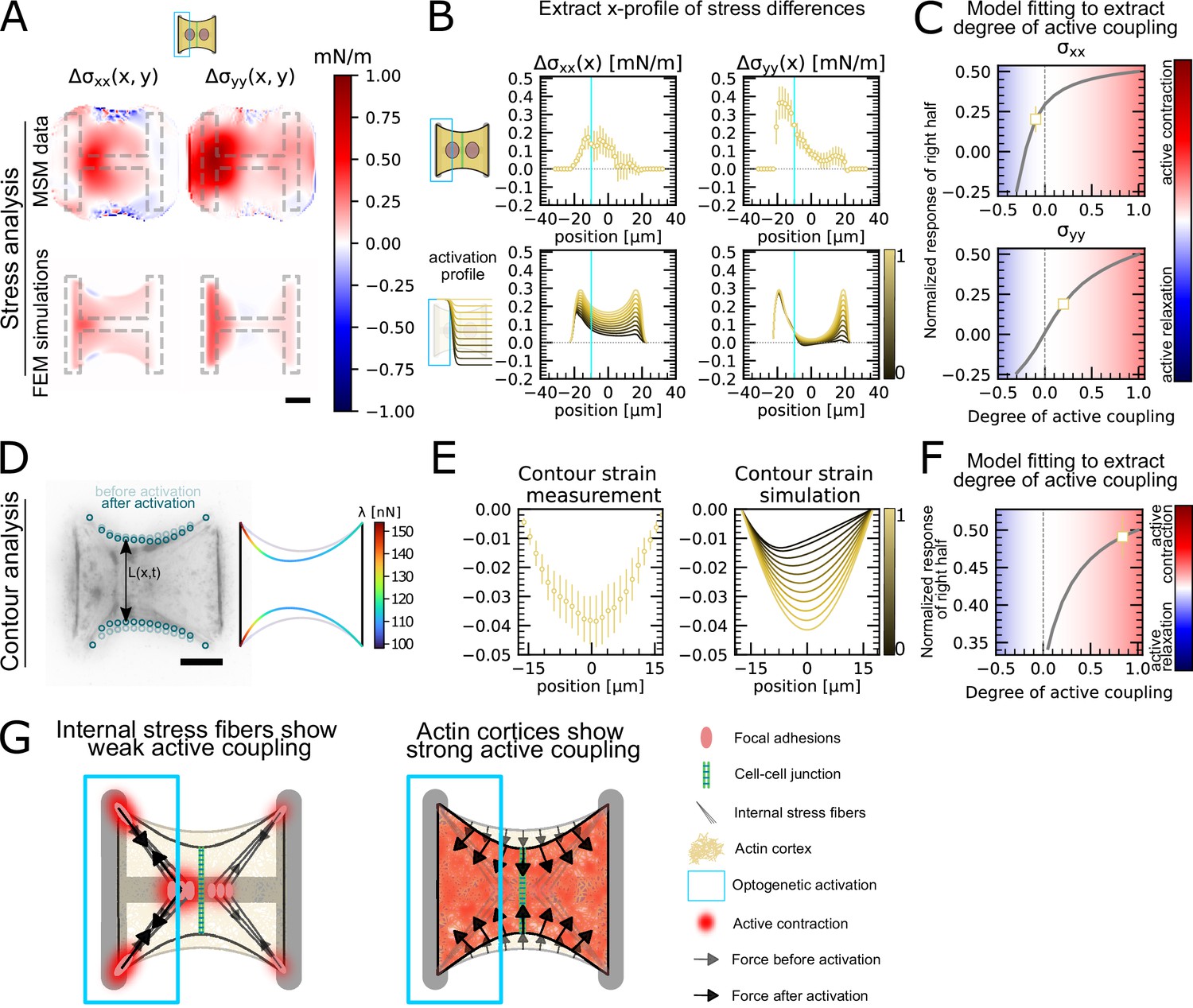
Stress and contour modeling shows strong active coupling of actin cortices in doublets.
(A) Difference of average cell stress maps after and before photoactivation of cell doublets, calculated with monolayer stress microscopy (MSM) (top) and simulated with the FEM continuum model (bottom). Stress in x-direction is shown on the left, and stress in y-direction is shown on the right. (B) Average over the y-axis of the maps in (A). Data is shown as circles with the mean ± SEM. In the simulation, the right half of the cell was progressively activated to obtain the family of curves shown in the bottom. (C) Response of the right half (normalized by the total response), obtained from the model (gray line), as a function of the degree of active coupling. The experimental MSM value is placed on the curve to extract the degree of active response of the right cell in the experiment. (D) Contour analysis of the free stress fiber. In the experiment, the distance between the free fibers as a function of x is measured, as shown in the image on the left. An example for a contour model simulations is shown in the right. (E) The contour strain after photoactivation is calculated from the distance measurements shown in (D) by dividing the distance between the free stress fibers for each point in x-direction after and before photoactivation. Similarly to the FEM simulation, in the contour simulation, the right half of the contour is progressively activated to obtain the curve family shown in the right plot. (F) Response of the right half (normalized by the total response), obtained from the model (gray line), as a function of the degree of active coupling. The experimental strain value is placed on the curve to extract the degree of active response of the right cell in the experiment. (G) A cartoon showing our interpretation of the results shown in panels (A–F). The traction force analysis only measures forces that are transmitted to the substrate, which are dominated by the activity of the stress fibers. The contour of the free fiber is determined by the activity of the actin cortex and the free stress fiber. Thus, the strong active coupling in the contour suggests strong active coupling of the cortices and the comparatively weak active coupling of the forces suggests a weak active coupling of the stress fibers. The figure shows data from n = 17 doublets from N = 2 samples. All scale bars are long.
Figure 5 with 1 supplement
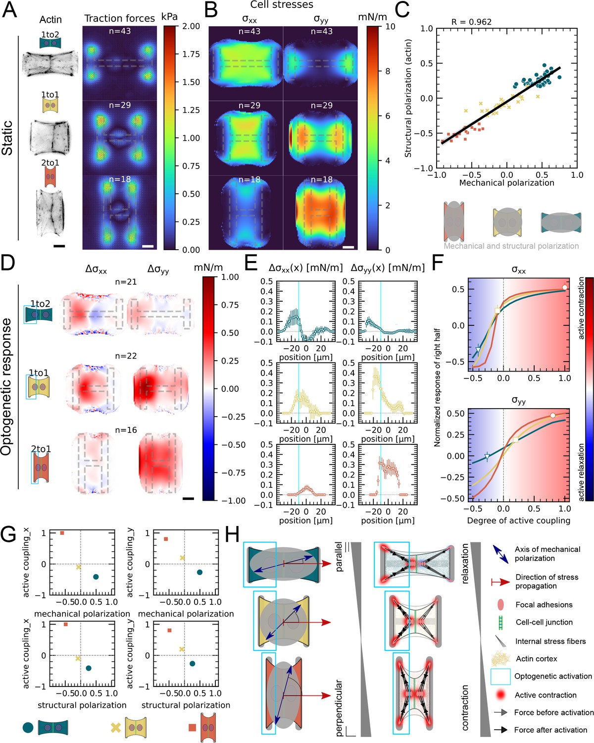
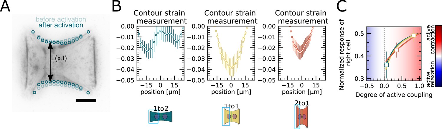
Mechanical stresses transmit most efficiently perpendicularly to the axis of mechanical and structural polarization in doublets.
(A) Actin images (left) and average traction stress and force maps (right) of cell doublets on H-patterns with different aspect ratios (1 to 2, 1 to 1, and 2 to 1). (B) Average cell stress maps calculated by applying a monolayer stress microscopy algorithm to the traction stress maps. (C) Correlation plot of mechanical and structural polarization. The black line shows the linear regression of the data, and the shaded area shows the 95% confidence interval for this regression. The R-value shown corresponds to the Pearson correlation coefficient. (D) Stress maps of the difference of xx-stress (left) and yy-stress (right) before and after photoactivation. (E) Average over the y-axis of the maps in (D). Data is shown as circles with the mean ± SEM. (F) Response of the right half (normalized by the total response), obtained from the model (gray line), as a function of the degree of active coupling. The experimental monolayer stress microscopy (MSM) value is placed on the curve to extract the degree of active response of the right cell in the experiment. All scale bars are long. (G) The degree of active coupling plotted against the average mechanical and structural polarization. (H) A cartoon showing our interpretation of the data shown in panels (A–F). The relative response of the right cell in response to the activation of the left cell varies strongly in the different aspect ratios. In the 1 to 2 doublet, where polarization and transmission direction are aligned, the right cell relaxes, whereas in the 2 to 1 doublet, where the polarization axis is perpendicular to the transmission direction, the right cell contracts almost as strongly as the left cell. The figure shows data from n = 43 1 to 2 doublets from N = 6 samples, n = 29 1 to 1 doublets from N = 2 samples, and n = 18 2 to 1 doublets from N = 3 samples. For the analysis of the optogenetic data, doublets with unstable stress behavior before photoactivation were excluded. All scale bars are long.
Figure 5—figure supplement 1
Contour strain measurements of doublets with varying aspect ratios.
(A) Contour analysis of the free stress fiber. In the experiment, the distance between the free fibers as a function of x is measured, as shown in the image on the left. (B) The contour strain after photoactivation is calculated from the distance measurements shown in (A), by dividing the distance between the free stress fibers for each point in x-direction after and before photoactivation. (C) Response of the right half (normalized by the total response), obtained from the model (solid lines), as a function of the degree of active coupling. The experimental strain value is placed on the curve to extract the degree of active response of the right cell in the experiment.
Figure 6 with 1 supplement
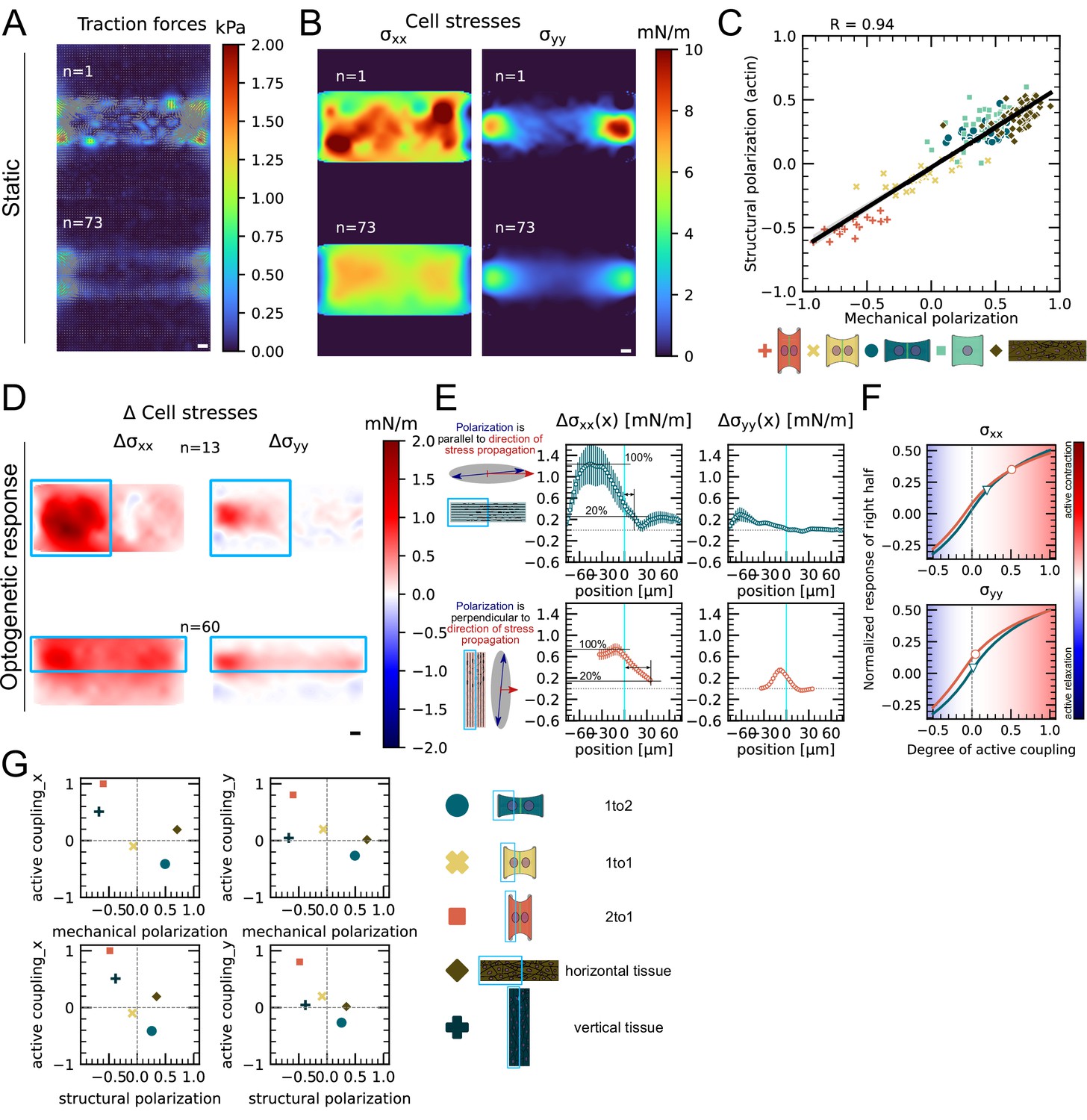
Mechanical stresses transmit most efficiently perpendicularly to the axis of mechanical and structural polarization in small monolayers.
(A) Representative (top) and average (bottom) maps of traction forces and stresses of a small monolayer on rectangular micropattern. (B) Representative example and average cell stress maps calculated by applying a monolayer stress microscopy algorithm to the traction stress maps. (C) Correlation plot of mechanical and structural polarization across all conditions. The black line shows the linear regression of the data, and the shaded area shows the 95% confidence interval for this regression. The R-value shown corresponds to the Pearson correlation coefficient. (D) Stress maps of the difference of xx-stress (left) and yy-stress (right) before and after photoactivation. (E) Average over the y-axis of the maps in (D). Data is shown as circles with the mean ± SEM. (F) Response of the right half (normalized by the total response), obtained from the model (gray line), as a function of the degree of active coupling. The experimental monolayer stress microscopy (MSM) value is placed on the curve to extract the degree of active response of the right cell in the experiment. (G) The degree of active coupling plotted against the average mechanical and structural polarization. All scale bars are long. The figure shows data from n = 13 tissues from N = 2 samples photoactivated on the left and from n = 60 tissues from N = 3 samples photoactivated on the top. All scale bars are long.
Figure 6—figure supplement 1
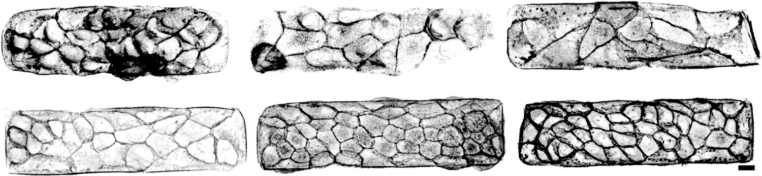
Phalloidin stainings of actin structures of small tissues.
Scale bar is long.
Appendix 1—figure 1
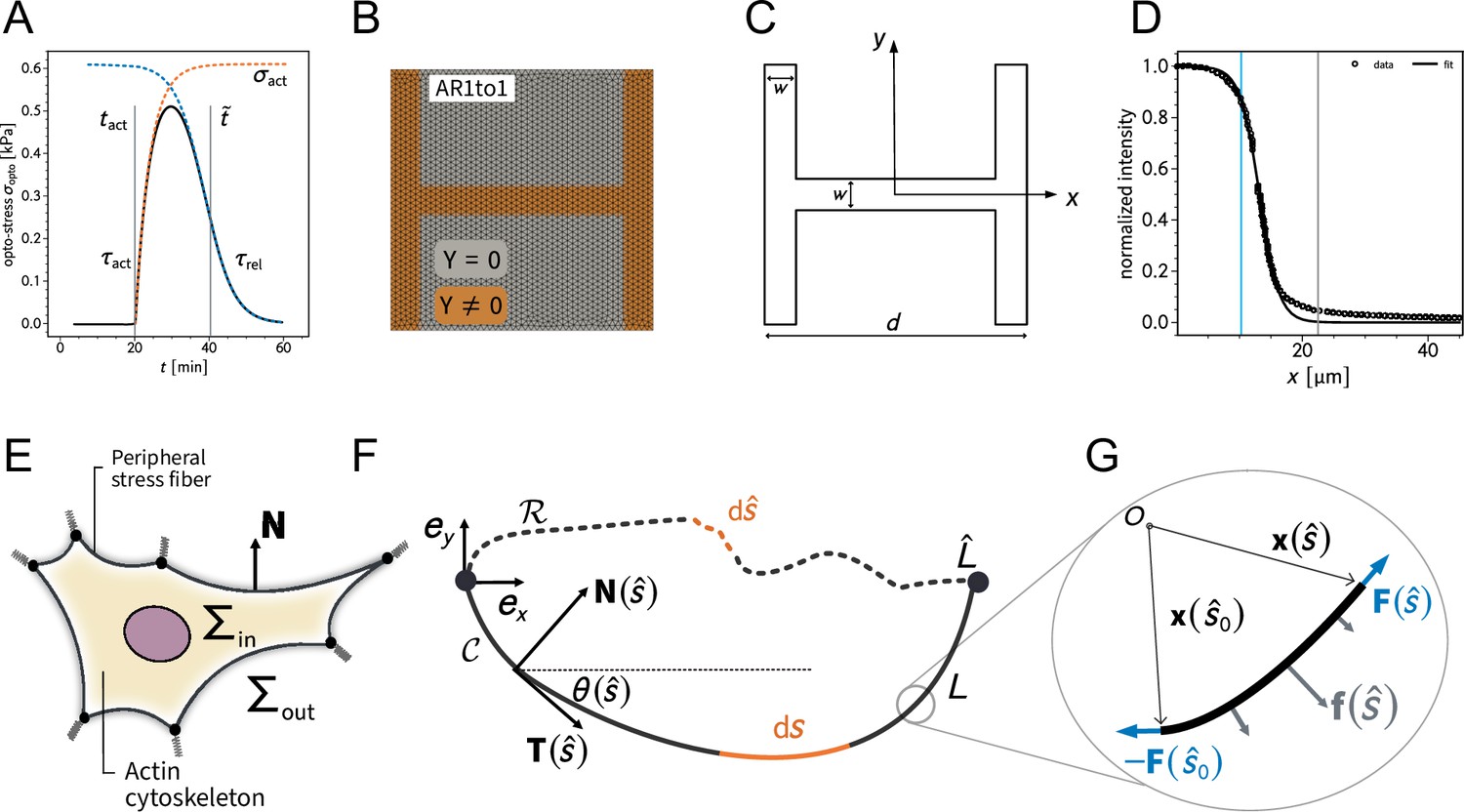
Overview of the 2D finite element simulation and the notation for the contour model.
(A) shows the shape of the by optogenetic-induced time-dependent stress. (B) depicts the finite element mesh created with GMSH. The spring stiffness density is nonzero on the brown part of the domain. (C) is a schematic illustration of the relevant parameters to define the adhesion geometry. (D) shows the experimentally measured intensity profile of the light pulse used for photoactivation. The gray line indicates the center of the pattern (measured from left to right) while the blue line marks the inflection point of the sigmoidal fit function. (E) is a schematic illustration of the relevant quantities in the contour-based description of cellular adhesion. (G, F) explain the relevant mathematical quantities to describe the equilibrium shape of a fiber subject to external loads.
Appendix 1—figure 2
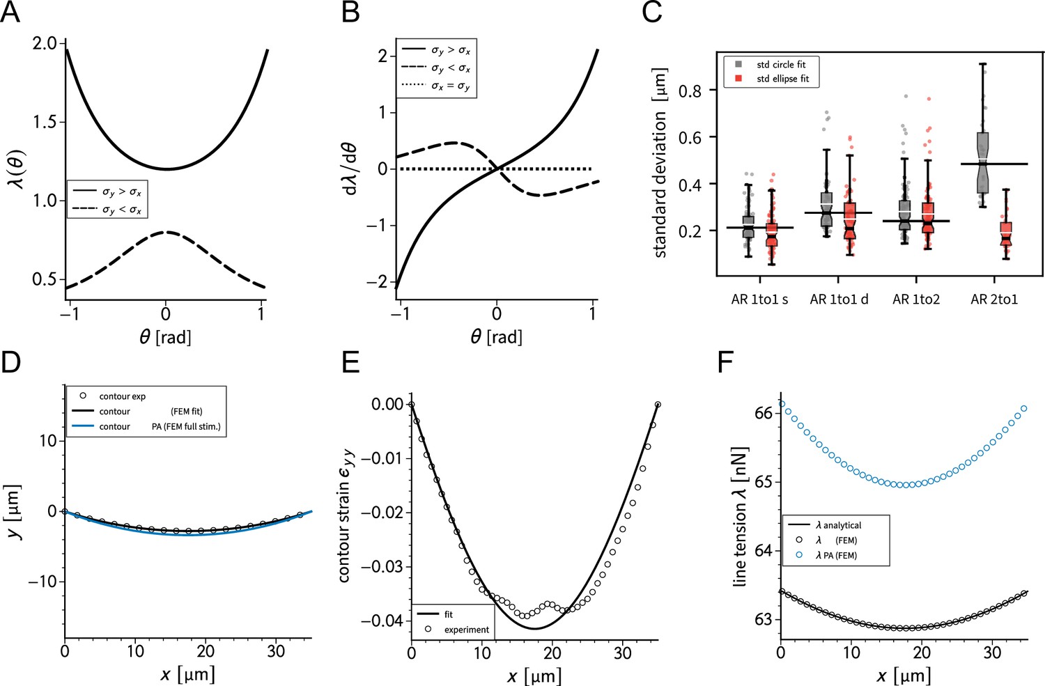
Calibration check for the contour model.
(A, B) show the predicted line tensions and the derivative with respect to the turning angle based on the analytical solution for different values of and . (C) compares the circle and ellipse fit of the contour of the cells for different pattern aspect ratios. (D) shows a generic cell contour for the doublet before and during photo-activation. The experimentally contour strain in -direction with the respective fit from simulations and the corresponding line tensions are shown in (E) and (F), respectively.
Appendix 1—figure 3
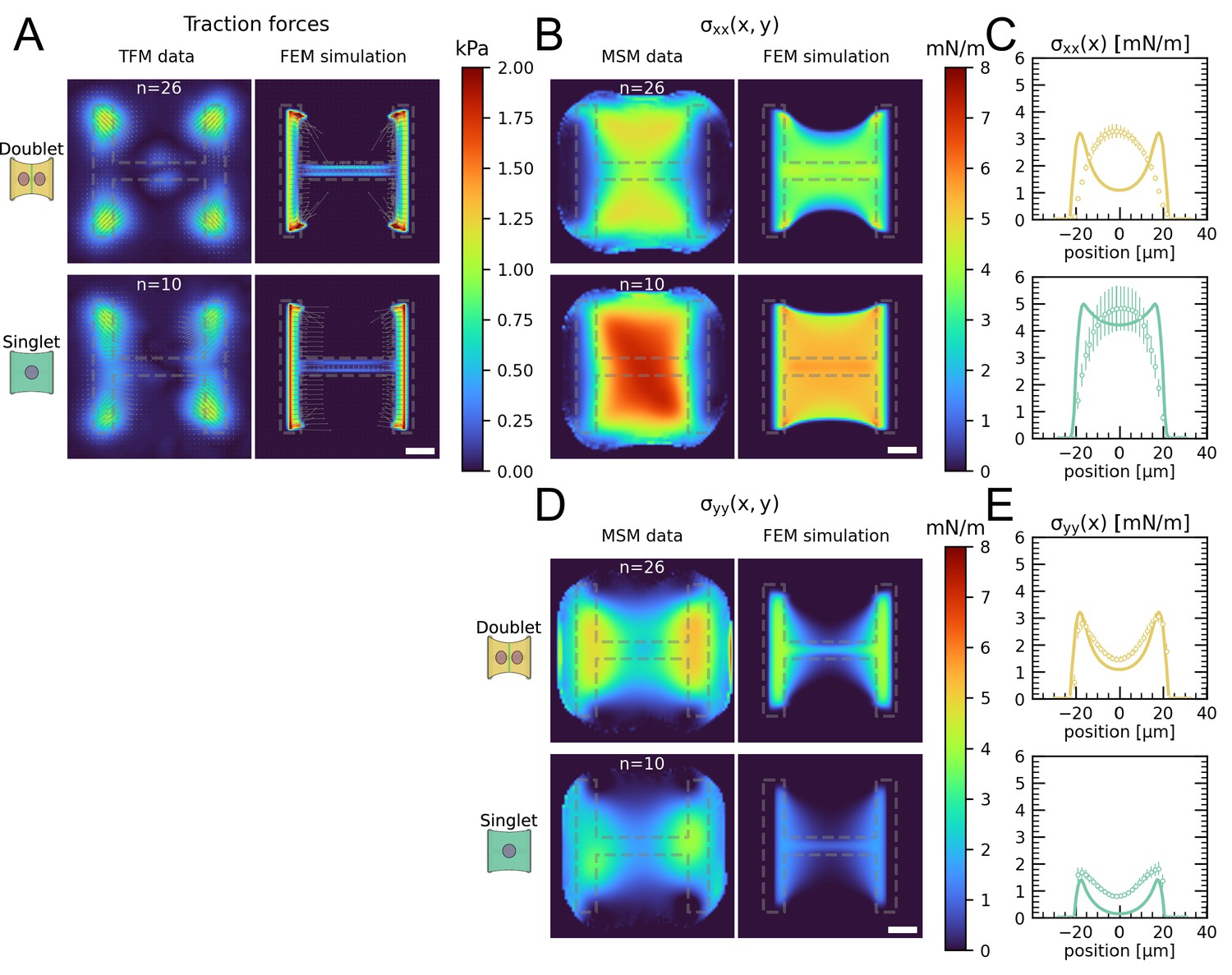
Comparison of traction forces and stress distribution between experiment and finite element simulation.
(A) Average traction stress and force maps of cell doublets (top) and singlets (bottom) on H-patterns on the left and corresponding traction stress and force maps from the FEM simulation. (B, D) Average cell stress maps of cell doublets (top) and singlets (bottom) on H-patterns on the left and corresponding cell stress maps from the FEM simulation. (C, E) Average over the y-axis of the maps in (B) and (D). Data is shown as circles with the mean ± SEM, the solid line corresponds to the FEM simulations. All scale bars are long.
Appendix 1—figure 4
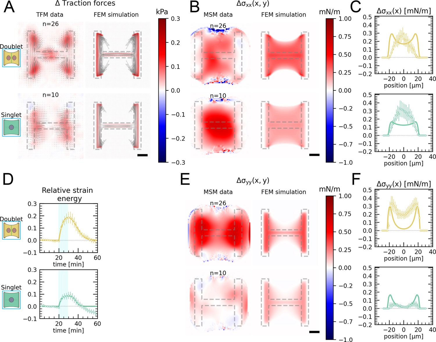
Comparison of traction forces stress distribution and strain energy between experiment and finite element simulation for global photoactivation.
(A) Average traction stress and force map difference before and after photoactivation of cell doublets (top) and singlets (bottom) on H-patterns on the left and corresponding traction stress and force maps from the FEM simulation. (B, E) Average cell stress map difference before and after photoactivation of cell doublets (top) and singlets (bottom) on H-patterns on the left and corresponding cell stress maps from the FEM simulation. (C, F) Average over the y-axis of the maps in (B) and (D). Data is shown as circles with the mean ± SEM, the solid line corresponds to the FEM simulations. (D) Relative strain energies of doublets (top) and singlets (bottom) with global photoactivation. One frame per minute was acquired for 60 min, and cells were photoactivated with one pulse per minute for 10 min between minute 20 and minute 30. Strain energy curves were normalized by first subtracting the individual baseline energies (average of the first 20 min) and then dividing by the average baseline energy of all cell doublets/singlets in the corresponding datasets. Data is shown as circles with the mean ± SEM, and the result of an FEM simulation is shown as a solid line. All scale bars are long.
Author response image 1

Author response image 2
Author response image 3

(a) Composite brightfield image of opto-MDCK cells spreading on H-patterns. Fully spread doublets are marked with a white frame. (b) Graph shows number of fully spread doublets over time from one experiment on 20 kPa and one experiment on 40 kPa polyacrylamide gels.
Videos
Animation 1
Actin + traction forces (left) and relative strain energy (right) over time of a globally photoactivated doublet.
Animation 2
Nine examples of globally photoactivated doublets.
Actin is shown in black, traction forces are overlaid as colored arrows, the tracked contour in blue circles, the tangents in white dashed lines, and the fitted ellipse in green.
Animation 3
Nine examples of globally photoactivated singlets.
Actin is shown in black, traction forces are overlaid as colored arrows, the tracked contour in blue circles, the tangents in white dashed lines, and the fitted ellipse in green.
Animation 4
Actin + traction forces (left), traction force map (center), and relative strain energy divided in left (blue) and right (orange) half (right) over time of a locally photoactivated doublet.
Animation 5
Actin + traction forces (left), traction force map (center), and relative strain energy divided in left (blue) and right (orange) half (right) over time of a locally photoactivated singlet.
Animation 6
Average traction force maps (top) and relative strain energy divided in left (bright) and right (dark) half (right) over time of locally photoactivated 1 to 2 (blue), 1 to 1 (yellow), and 2 to 1 doublets (red).
Animation 7
Cry2 distribution with photoactivation of left cell in a doublet with increasing power densities.
First pulse: ; second pulse: ; third pulse: ; fourth pulse: ; fifth pulse: ; sixth pulse: .
Animation 8
Cropped images from brightfield timelapse of doublets forming on H-patterns.
Tables
Appendix 1—table 1
Fixed parameters for the two-dimensional finite element simulation.
| Fixed parameter | Value |
|---|---|
| Substrate | |
| Young’s modulus of the substrate, | |
| Poisson’s ratio of the substrate, | |
| Thickness of the substrate, | |
| Cell | |
| Young’s modulus of cell, | |
| Viscosity of the cell, | |
| Effective thickness of the cell, | |
| Poisson’s ratio of the cell, | |
| Length of the cell, | |
Appendix 1—table 2
Fit parameters as obtained by the two-dimensional finite element simulation.
| Fit parameter | Singlet | Doublet |
|---|---|---|
| Baseline | ||
| Background stress component, | ||
| Background stress component, | ||
| Full opto-stimulation | ||
| Active stress, | ||
| Activation time scale, | ||
| Relaxation time scale, | ||
| Centroid, | ||
Appendix 1—table 3
Fit parameters for baseline fit of AR 1 to 2 and AR 2 to 1 doublets.
The background stress was obtained from a fit of the model to the strain energy baseline. Based on the values for the mechanical polarization reported in Figure 5G, we used for AR 1 to 2 and for AR 2 to 1. Together with the fitted values for we deduced from Equation (17).
| Fit parameter | AR 1 to 2 | AR 2 to 1 |
|---|---|---|
| Baseline | ||
| Background stress component, | ||
| Background stress component, | ||
Appendix 1—table 4
Fixed parameters used in the qualitative study of fluidization.
The order of magnitude for was set in accordance with the values reported in Oakes et al., 2017.
| Fixed parameter | Value |
|---|---|
| Young’s modulus of the substrate, | |
| Poisson’s ration of the substrate, | |
| Effective substrate thickness, | |
| Lateral cell size, | |
| Young’s modulus of the cell, | |
| Viscosity of the cell, | |
| Effective thickness of the cell, | |
| Background stress, | |
| Spring stiffness density, |
Appendix 1—table 5
Fixed and optimized parameters for the contour shape analysis by means of the contour finite element simulation.
| Parameter | Value |
|---|---|
| Fixed | |
| Surface tension component, | |
| Surface tension component, | |
| Semi-axis, | |
| Semi-axis, | |
| One-dimensional elastic modulus, | |
| Contour fit | |
| Active line tension, | |
| Strain fit | |
| Relative surface tension increase, | |
| Relative surface tension increase, | |
Additional files
Download links
A two-part list of links to download the article, or parts of the article, in various formats.
Downloads (link to download the article as PDF)
Open citations (links to open the citations from this article in various online reference manager services)
Cite this article (links to download the citations from this article in formats compatible with various reference manager tools)
Force propagation between epithelial cells depends on active coupling and mechano-structural polarization
eLife 12:e83588.
https://doi.org/10.7554/eLife.83588


