Behavioral discrimination and olfactory bulb encoding of odor plume intermittency
- Interdepartmental Neuroscience Program, Yale University, United States
- John B. Pierce Laboratory, United States
- Department of Neuroscience, Yale School of Medicine, United States
- Department of Civil, Environmental and Architectural Engineering, University of Colorado, United States
Figures
Figure 1 with 1 supplement

Intermittent odor plume stimuli and olfactometer design.
(A) Graphical illustration of the intermittency measure. Intermittency (I) is the fraction of time an odorant concentration is above a threshold (0.1*C0, where C0 refers to the time-averaged source concentration). In a turbulent plume I drops as a function of distance. Hence, upstream (near the odor source) I tends to be large (here I=0.6) compared to downstream, distant from the odor source (here I=0.09). A steady signal has a high intermittency, and a sporadic signal has a low intermittency. (B) Odor delivery system used to deliver methyl valerate and 2-heptanone. Two counterbalanced proportional valves maintained constant flow rate. (C) Example of odor concentration (red) and flow rate (black) on a single trial. (D) Cross-correlation between photoionization detector (PID) measurement (odor concentration) and the command voltage driving movement of the odor proportional valve. Maximum correlation coefficient is 0.872 ± 0.119 at a lag of 160 ms (n=8643 trials). (E) Example correlation between the trial intermittency value measured from the PID reading vs the intermittency value measured from the voltage command for one session (n=64 trials). Linear regression: y=1.09x+0.023, r2=0.996, p<0.0001. (F) Example traces of odor concentration at gain 1 (darker colors) and gain 0.5 (lighter colors) for naturalistic, binary naturalistic, and square-wave stimuli. (G) Median r2 of the correlation between voltage intermittency and PID intermittency for sessions of naturalistic (red), binary naturalistic (orange), and square-wave (blue) stimuli (n=48 sessions per stimulus type, naturalistic median = 0.945 interquartile range [IQR]=[0.937–0.949], binary naturalistic median = 0.998 IQR=[0.997–0.999], square-wave median = 0.987 IQR=[0.982–0.991]).
Figure 1—figure supplement 1
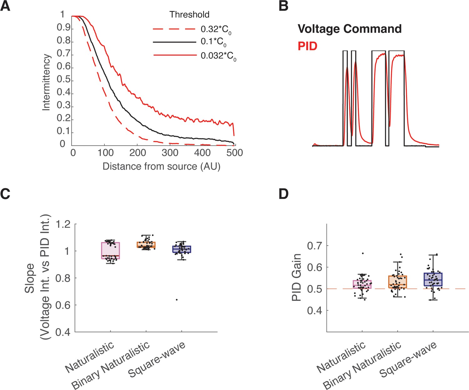
Additional information on intermittent odor plume stimuli and intermittency calculation.
(A) Odor intermittency as a function of distance downstream from odor source. Three odor concentration thresholds used to calculate intermittency are represented. Black line displays an exponential decrease of intermittency, based on the 0.1*C0 threshold (C0 is source concentration) used in this paper. The surrounding lines show similar exponential relationship when thresholds were three times lower (red dashed, bottom), or three times higher (red solid, top), but with an expected downstream shift. X-axis units are pixel number downstream from the upstream release location and can be interpreted as release distance of arbitrary unit (AU, i.e. scale-free), but were based on a flow chamber of roughly 1 m downstream size. (B) Example trial of voltage command and resulting photoionization detector (PID) reading. (C) Median slope of the correlation between voltage intermittency and PID intermittency for sessions of naturalistic (red), binary naturalistic (orange), and square-wave (blue) stimuli (n=48 sessions per stimulus type, naturalistic median = 0.96 interquartile range [IQR]=[0.94 1.06], binary naturalistic median = 1.04 IQR=[1.03 1.06], square-wave median = 1.01 IQR=[0.99 1.04]). (D) Median PID gain on 0.5 gain trials (n=48 sessions per stimulus type, naturalistic median = 0.52 IQR=[0.50 0.54], binary naturalistic median = 0.52 IQR=[0.50 0.56], square-wave median = 0.54 IQR=[0.51 0.57]). One sample t-test with Ho:μ=0.5, p>0.05.
Figure 2 with 1 supplement
Mice can discriminate between fluctuating odor stimuli based on intermittency values.
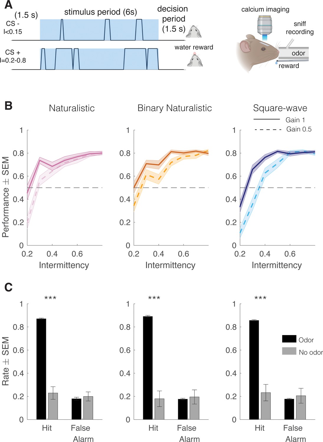
(A) Go/No-Go intermittency discrimination task structure. Animals are presented with a 6 s odor stimulus following a 1.5 s delay and after the odor presentation have a 1.5 s decision period during which, if they lick for a CS+, they receive a water reward, and if they lick for a CS-, they receive a punishment in the form of an increased ITI. Left: Imaging and odor delivery setup. Mice are delivered odor through a tube in front of their nose and sniffing is recorded through a pressure sensor inserted into the odor tube. Glomerular activity in the dorsal olfactory bulb is imaged using wide-field calcium imaging. (B) Mouse performance on intermittency discrimination task. At gain 1, mice perform significantly above chance at intermittency values of 0.3 and above (one-tailed t-test, Bonferroni correction, p<0.0001, n=48 sessions) for all stimulus types. At gain 0.5, mice perform above chance at intermittency values 0.4 and above, naturalistic and square-wave, 0.5 and above, binary naturalistic (one-tailed t-test, Bonferroni correction, p<0.0001, n=48 sessions). (C) Hit rates (HR) and false alarm (FA) rates of mice performing the intermittency discrimination task with and without odor. Two-sample t-tests. Naturalistic: μ HROdor=0.87±0.006, μHRNoOdor=0.23±0.055, p<0.0001, μFAOdor=0.18±0.013, μFANoOdor=0.20±0.039, p=0.64, binary naturalistic: μHROdor=0.89±0.009, μHRNoOdor=0.18±0.068, p<0.0001, μFAOdor=0.18±0.008, μFANoOdor=0.19±0.061, p=0.75, square-wave: μHROdor=0.86±0.007, μHRNoOdor=0.23±0.071, p<0.0001, μFAOdor=0.18±0.006, μFANoOdor=0.21±0.065, p=0.67.
Figure 2—figure supplement 1
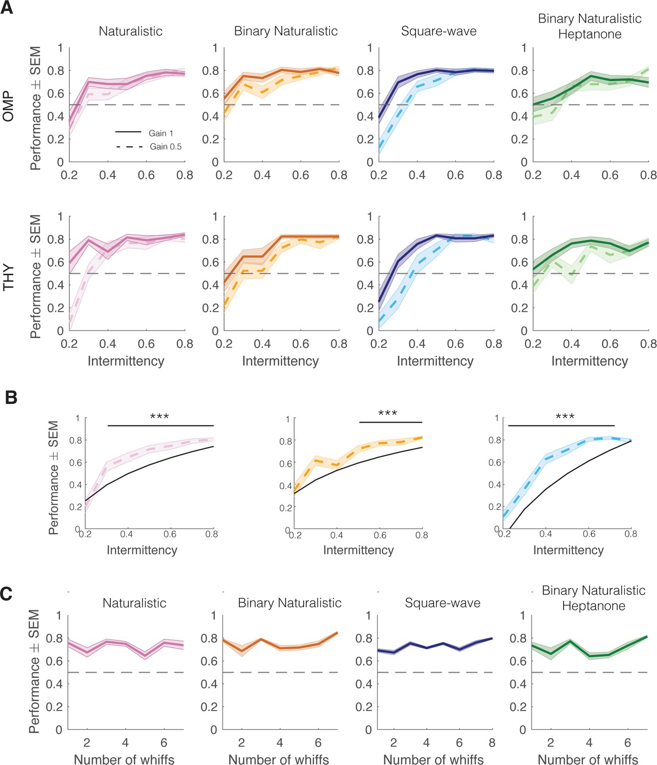
Intermittency discrimination performance by genotype, odor, and whiff number.
(A) Performance curves by genotype (OMP-GCaMP6f and THY1-GCaMP6f). (B) Performance on 0.5 gain trials (dotted colored line) and predicted performance of odor integration strategy at 0.5 gain (black line). One-tailed, one-sample t-test with Bonferroni correction. Ho: µ Performance=predicted performance. Naturalistic intermittency≥0.3, p<0.0001; naturalistic intermittency≥0.5, p<0.0001; square-wave intermittency≤0.8, p<0.0001. (C) Performance by number of whiffs in odor stimulus. Spearman correlation, p>0.05.
Figure 3 with 2 supplements

Estimated perceived intermittency differs based on trial outcome.
(A) Example photoionization detector (PID) trace (red) and pressure sensor trace (black), and blue lines correspond to inhalation periods. Left: Example estimated perceived odor trace (PID trace sampled during inhalation periods). (B) Average cumulative estimated perceived intermittency (based on estimated perceived odor) across trial time for trials with intermittency values between 0.1 and 0.8 for binary naturalistic (n=1362 trials, left) and square-wave (n=1341 trials, right). (C) Example PID reading (red), sniff trace (black), lick trace (blue) during an example high intermittency trial (top, intermittency = 0.8) and low intermittency trial (bottom, intermittency = 0.3). Gray area indicates 6 s odor stimulus period. Following the stimulus period is the decision period where a water reward is delivered if animals lick for a CS+ (indicated by the water droplet). (D) Time of first lick binned by intermittency using both odor intermittency (blue) and estimated perceived intermittency (black) for binary naturalistic (n=1362 trials, left) and square-wave (n=1341 trials, right). (E) Estimated perceived intermittency vs odor intermittency on hit and miss CS+ trials (n=48 sessions). (F) Right: Square-wave. Accuracy of linear classifier performance in predicting trial identity (CS+ or CS-) for trials of intermittency values between 0.2 and 0.8 (CS+) based on estimated perceived intermittency (gray to black lines). Shuffled control is shown in red. One-sided two-tailed t-test with Bonferroni correction. Left: Binary naturalistic, intermittency values ≥ 0.3, all times are significantly above shuffled control (black bar, p<0001). Intermittency values = 0.2, times ≥4 s are significantly above shuffled control (gray line, p<0001). Right: Square-wave, intermittency values ≥ 0.3, all times are significantly above shuffled control (black bar, p<0001). Intermittency values = 0.2, times ≥3 s are significantly above shuffled control (gray line, p<0001) (n=20 repeats per time bin).
Figure 3—figure supplement 1
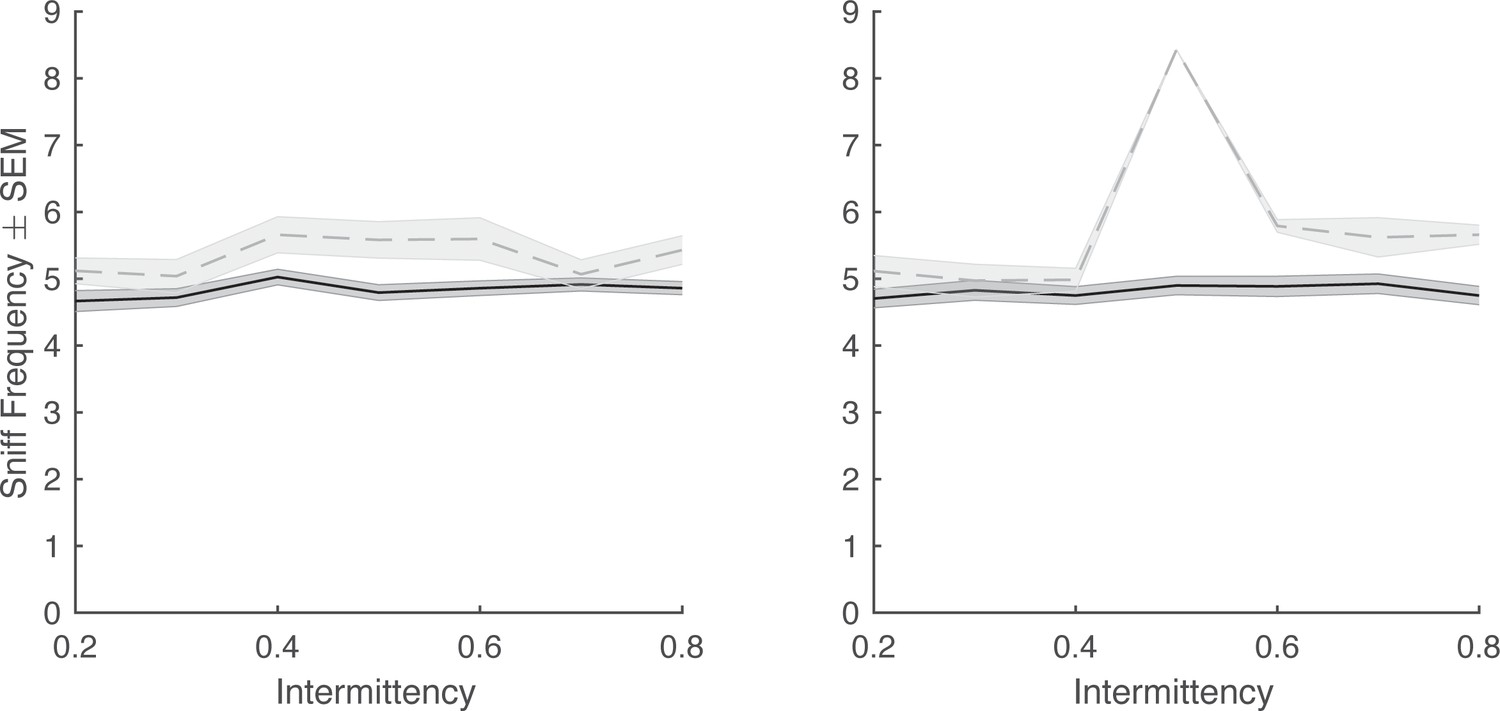
Average trial sniff frequency vs odor intermittency on hit and miss trials.
Miss trials are in gray and hit trials are in black. Left: Binary naturalistic. Right: Square-wave (n=48 sessions each, generalized linear model; sniff frequency~trial outcome*intermittency, p>0.05; note: only one session with miss trials for synthetic stimuli at intermittency = 0.5).
Figure 3—figure supplement 2
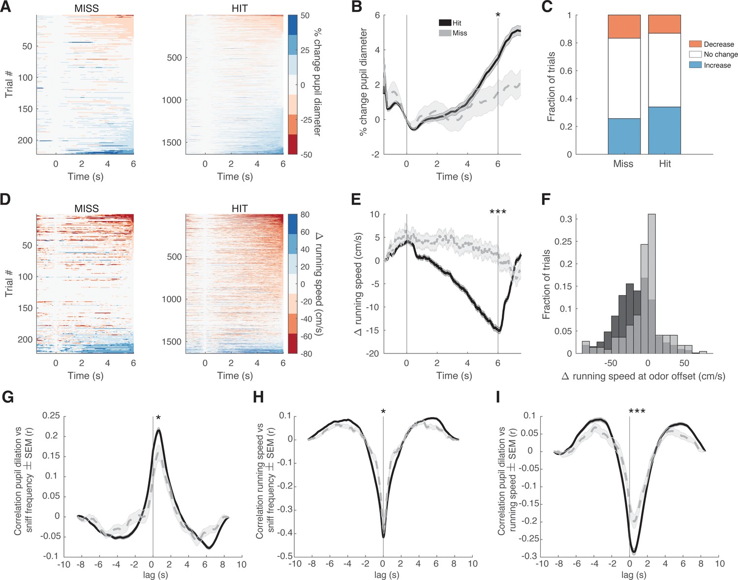
Pupil dilation and running speed differ between hit and miss trials.
For all graphs miss trials are in gray and hit trials are in black. (A) Heatmap of the % change in pupil diameter from odor onset (time 0 s) for miss and hit trials. (B) Average change in pupil diameter across trial time (odor onset is at time = 0 s and odor offset is at time = 6 s) for hit and miss trials. t-Test at odor offset, p<0.05. (C) Fraction of trials with an increase, decrease, or no change in pupil dilation at the time of odor offset. Miss: increase, 25.7%; decrease, 16.7%; no change, 57.7%. Hit: increase, 34%; decrease, 13.1%; no change, 52.9%. (D) Heatmap of the change in running speed (cm/s) from odor onset (time 0 s) for hit and miss trials. (E) Average change in running speed across trial time (odor onset is at time = 0 s and odor offset is at time = 6 s) for hit and miss trials. t-Test at odor offset, p<0.0001. (F) Histogram of the change in running speed at odor offset for all trials. Two-sample Kolmogorov-Smirnov test, p<0.0001. (G) Cross-correlation of between pupil dilation and instantaneous sniff frequency during odor delivery period. Two-sample t-test at peak, p<0.05. (H) Cross-correlation between running speed and instantaneous sniff frequency during odor delivery period. Two-sample t-test at peak, p<0.05. (I) Cross-correlation between pupil dilation and running speed during odor delivery period. Two-sample t-test at peak, p<0.0001. In all cases a positive lag indicates a delay in the first parameter listed.
Figure 4 with 1 supplement

Spatial mapping of glomerular response properties across intermittency.
(A) Example low intermittency trial (top) and a high intermittency trial (bottom). Photoionization detector (PID) trace (red), sniff trace (black), and deconvolved ΔF/F traces of two example glomeruli (left, color coded based on odor correlation color bar, right). Example spatial maps of glomeruli color coded based on glomerular response correlation with odor. Two example glomeruli shown in the left traces are labeled, middle. Cross-correlation between deconvolved ΔF/F and odor for each glomerulus for example trials, right. (B) Glomerular odor correlation organized based on glomerulus anterior to posterior and medial to lateral location in the dorsal olfactory bulb (low intermittency example, top two graphs; high intermittency example, bottom two graphs). Low intermittency: M-L r=0.34, A-P r=0.58; high intermittency: M-L r=0.58, A-P r=0.62. (C) Correlation coefficient of glomerular odor correlation in each dimension (based on graphs in B for all trials). Trial averages are separated by odor intermittency value (colorbar). M-L:μint0.1-0.2=0.23, μint0.3-0.4=0.33, μint0.5-0.6=0.35, μint0.7-0.8=0.37; A-P: μint0.1-0.2=0.46, μint0.3-0.4=0.48, μint0.5-0.6=0.48, μint0.7-0.8=0.50. (D) Spatial odor map (z-score amplitude, open circle) and spatiotemporal odor map (T75, gray) (for methyl valerate). M-L: μz-score(Amplitude)=0.18, μT75=-0.33; A-P: μz-score(Amplitude)=0.37, μT75=-0.32. (E) Probability density function of T75 for all glomeruli and Gaussian curve fits for fast responding glomeruli cluster (dark gray) and slow responding glomeruli cluster (light gray) (top). Glomerulus odor correlation on trials with intermittency ≥0.7 vs glomerulus odor correlation on trials with intermittency ≤0.2. Fast responding glomeruli (low T75): y=0.65x–0.05, r2=0.77, p<0.0001. Slow responding glomeruli (high T75): y=0.29x+0.026, r2=0.53, p<0.0001 (n=244 glomeruli).
Figure 4—figure supplement 1
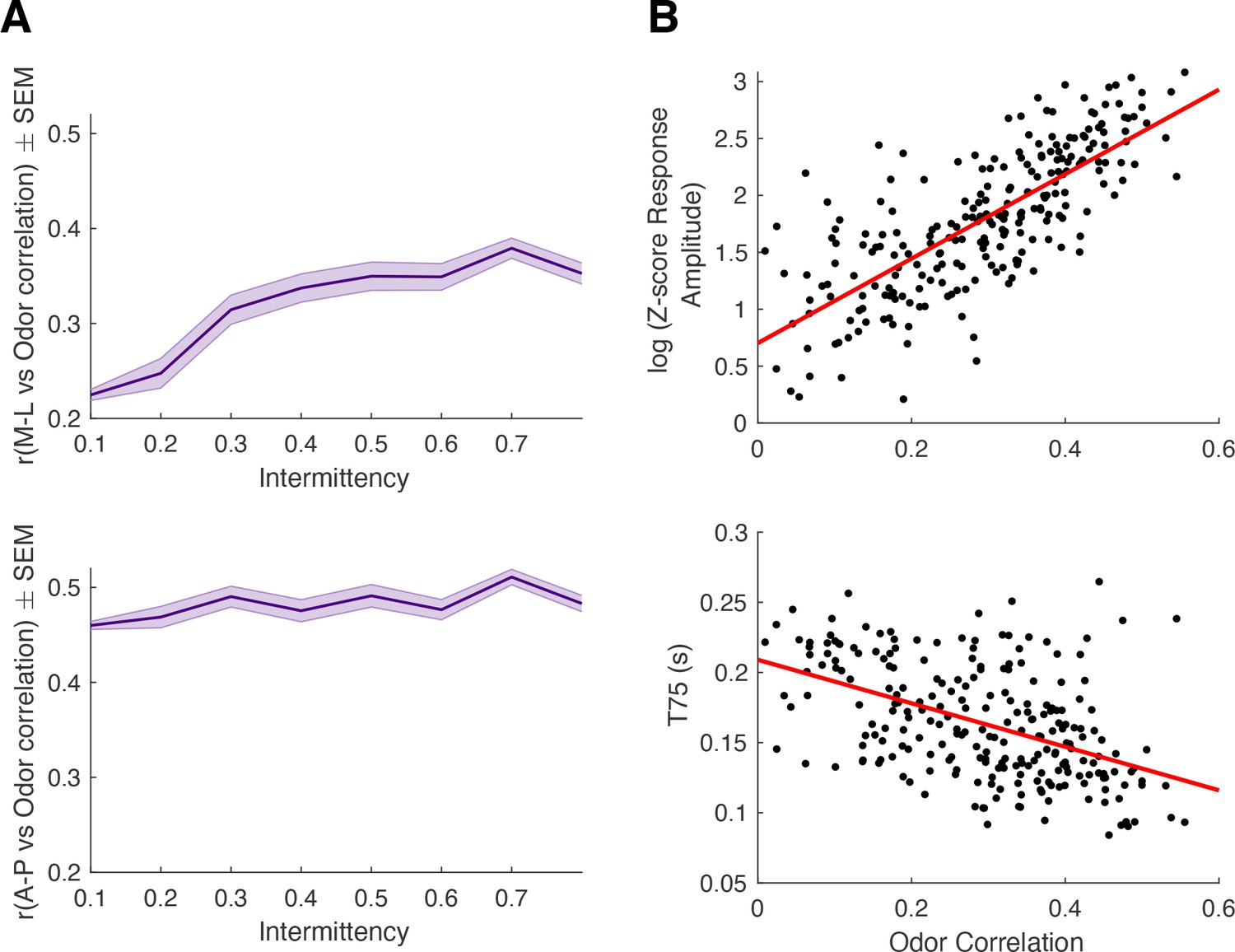
Relationship between odor correlation and spatial location, response amplitude, and t75.
(A) Spatial correlation of odor-response correlation in M-L (top) and A-P (bottom) directions across intermittency values. M-L linear regression: y=0.22x+0.21, p<0.0001, r2=0.08. A-P linear regression: y=0.05x+0.46, p<0.0001, r2=0.009. (B) log(z-score response amplitude) vs odor correlation (y=3.71x+0.70, r2=0.57, p<0.0001) and T75 vs odor correlation (y=−0.155x+0.21, r2=0.23, p<0.0001).
Figure 5 with 2 supplements

Intermittency encoded in olfactory sensory neuron (OSN) glomerular subpopulations.
(A) Color maps of glomerular intermittency binned by trial odor intermittency. Glomeruli are sorted by their glomerular intermittency (GI) slope (glomerular intermittency vs odor intermittency). Left: Example photoionization detector (PID) odor trace (red), raw sniff trace (black), and z-scored trace from one glomerulus. Horizontal line at y=2 indicates the threshold for glomerular intermittency quantification. (B) Left: Dendrogram for hierarchical cluster analysis. Gray indicates cluster 1 (37 glomeruli) and black indicates cluster 2 (191 glomeruli). Middle: Inter-glomerular correlation matrix. Colorbar corresponds to correlation coefficient (r) between two glomeruli (glomerular intermittency vs odor intermittency). Right: Colormap of normalized glomerular intermittency (normalized to individual glomerular maximum for clearer visualization of two clusters). Rows sorted by hierarchical clustering. (C) (i) Average slope of glomerular intermittency vs odor intermittency of cluster 1 and cluster 2 (μcluster1=–0.59±0.044, μcluster2=0.89±0.024). (ii) Average z-score response amplitude for glomeruli in cluster 1 and cluster 2 (μcluster1=6.3±0.55, μcluster2=7.5±0.33). (iii) Average T75 for glomeruli in cluster 1 and cluster 2 (μcluster1=179.2±5.6 ms, μcluster2=159.3±3 ms). (iv) Average correlation between glomerular deconvolved ΔF/F traces and PID reading for glomeruli in cluster 1 and cluster 2 (μcluster1=0.24±0.017, μcluster2=0.31±0.009). (D) Accuracy of linear classifier trained using 10, 15, 20, and 25 glomeruli (colorbar) at varying fractions of cluster 1 and cluster 2 glomeruli. (E) Left: Histogram of abs(GI slope) for all glomeruli. Black line indicates the bottom 25th percentile (0.53) and red line indicates the top 25th percentile (1.03). Right: True positive accuracy (CS+ predicted as CS+) of linear classifier trained on 0–50 glomeruli for glomeruli with the top 25th percentile of GI slopes (red) and the bottom 25th percentile of GI slopes. Dashed line indicates hit rate of animals on behavioral task (0.87).
Figure 5—figure supplement 1
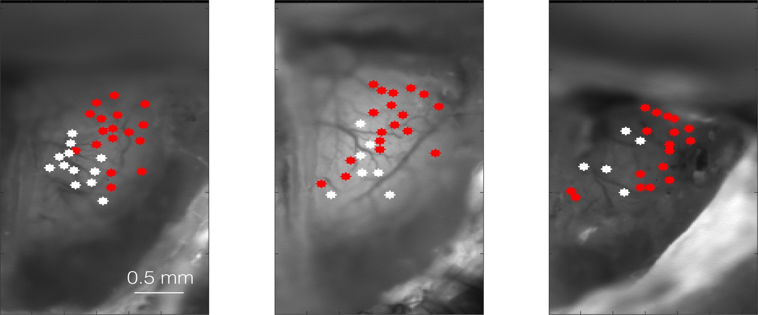
Example clusters from three different animals.
Cluster 1 (white) and cluster 2 (red)-identified glomeruli in three different OMP-GCaMP6f animals.
Figure 5—figure supplement 2
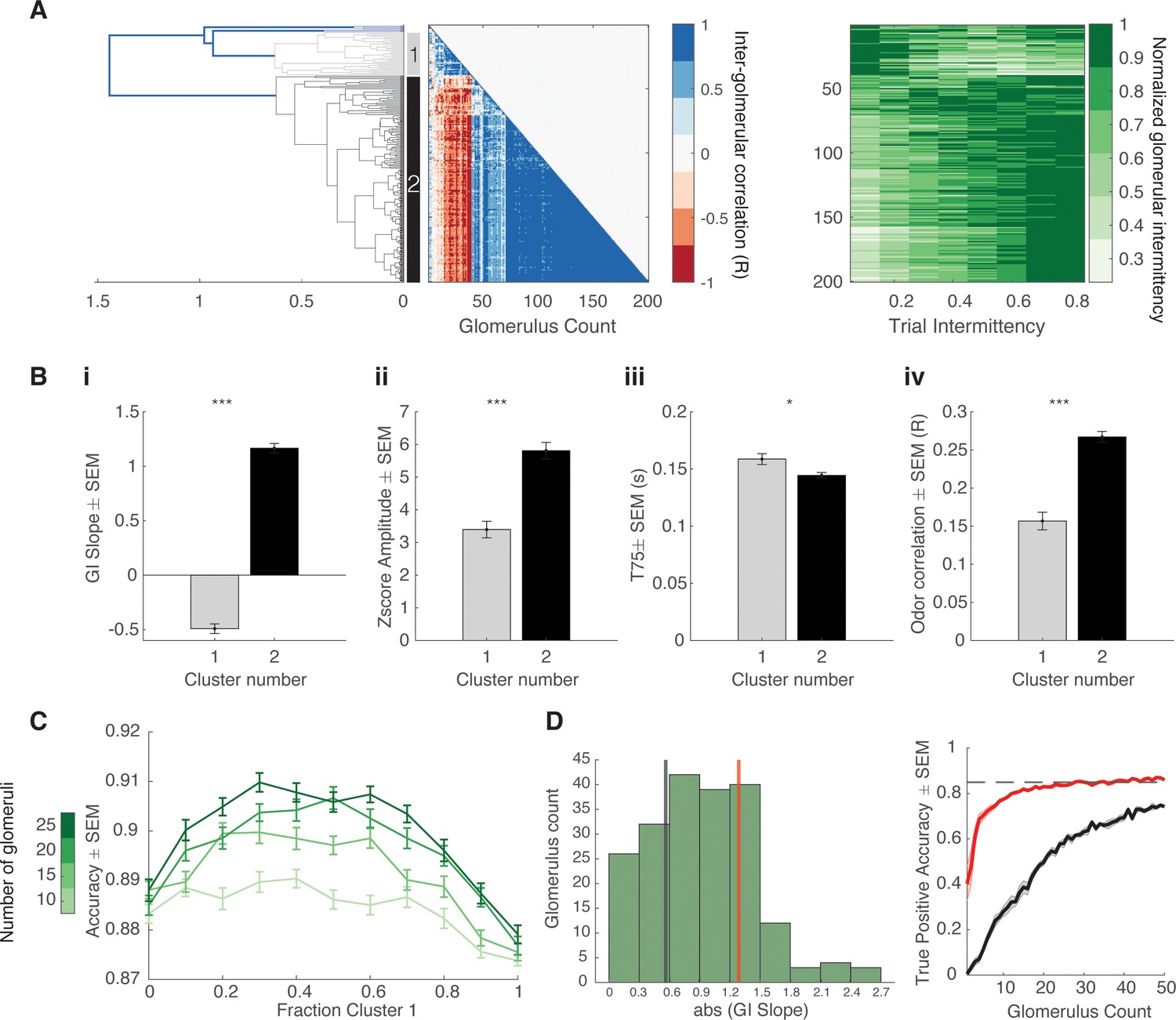
Intermittency encoded in mitral and tufted (M/T) cell glomerular subpopulations.
(A) Left: Dendrogram for hierarchical cluster analysis. Gray indicates cluster 1 (34 glomeruli) and black indicates cluster 2 (161 glomeruli). Middle: Inter-glomerular correlation matrix. Colorbar corresponds to correlation coefficient (r) between two glomeruli (glomerular intermittency vs odor intermittency). Right: Color map of normalized glomerular intermittency. Rows sorted by hierarchical clustering. (B) (i) Average slope of glomerular intermittency vs odor intermittency of cluster 1 and cluster 2 (μcluster1=–0.49±0.04, μcluster2=1.17±0.04). (ii) Average z-score response amplitude for glomeruli in cluser 1 and cluster 2 (μcluster1=3.4±0.25, μcluster2=5.82±0.25). (iii) Average T75 for glomeruli in cluster 1 and cluster 2 (μcluster1=158.611.6 ms, μcluster2=144.4±2.5 ms). (iv) Average correlation between glomerular deconvolved ΔF/F traces and PID reading for glomeruli in cluster 1 and cluster 2 (μcluster1=0.16±0.005, μcluster2=0.27±0.007). (C) Accuracy of linear classifier trained using 10, 15, 20, and 25 glomeruli (colorbar) at varying fractions of cluster 1 and cluster 2 glomeruli. (D) Left: Histogram of abs(GI slope) for all glomeruli. Black line indicates the bottom 25th percentile (0.56) and red line indicates the top 25th percentile (1.29). Right: True positive accuracy (CS+ predicted as CS+) of linear classifier trained on 0–50 glomeruli for glomeruli with the top 25th percentile of GI slopes (red) and the bottom 25th percentile of GI slopes. Dashed line indicates hit rate of animals on behavioral task (0.85).
Figure 6 with 2 supplements
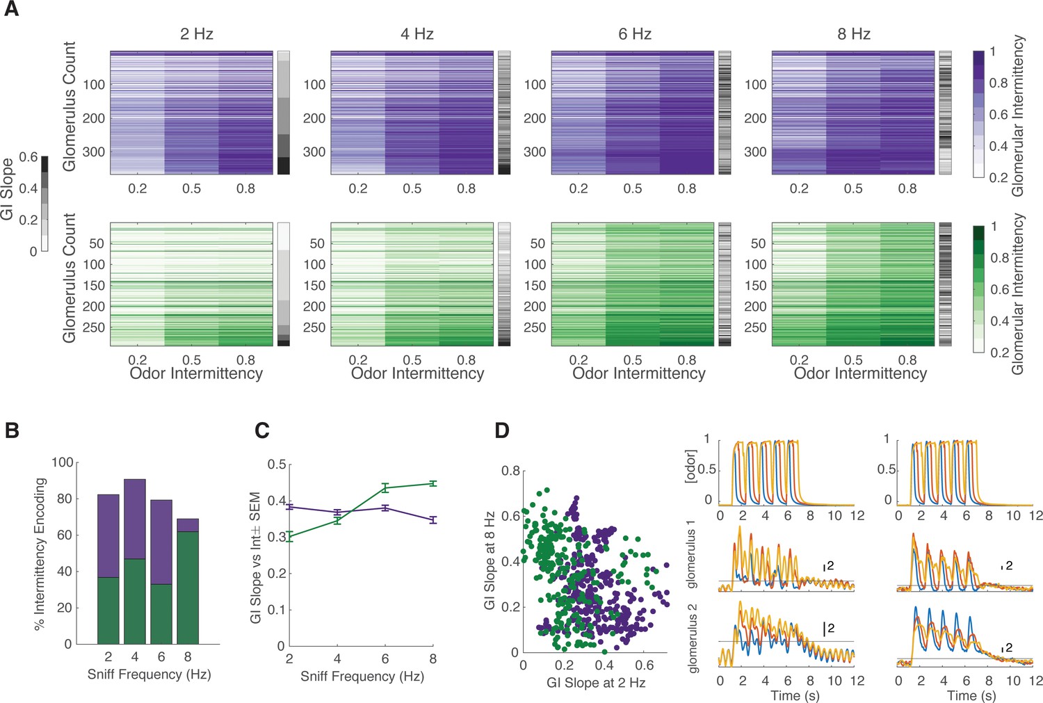
Effect of sniff frequency on glomerular representation of intermittency (methyl valerate).
For all graphs purple indicates olfactory sensory neurons (OSNs) (OMP-GCaMP6f) and green indicates mitral and tufted (M/T) cells (THY1-GCaMP6f). (A) Heatmap of glomerular intermittency (GI) across trials of 0.2, 0.5, and 0.8 odor intermittency values (colored heatmaps). Glomeruli are sorted based on their GI slope at 2 Hz. Gray bars next to heatmaps indicate the GI slope of each individual glomerulus. (B) % of intermittency encoding cells across sniff frequencies (OMP n=367 glomeruli, 7 mice; THY n=294 glomeruli, 6 mice). (C) GI slope as a function of sniff frequency. (D) Left: GI slope at 8 Hz as a function of GI slope at 2 Hz. Right: The top row shows example photoionization detector (PID) readings from square-wave trials with a fixed odor frequency of 0.83 Hz (5 pulses in 6 s) at intermittency values of 0.2 (blue), 0.6 (red), 0.8 (yellow). The first column represents averages from 2 Hz sniff frequency trials and the second column represents averages from 8 Hz sniff frequency trials. The second row shows example z-score deconvolved dF/F traces of a glomerulus with a low GI slope at 2 sniff frequency Hz and a high GI slope at 8 sniff frequency Hz. The last row shows example z-score deconvolved dF/F traces of a glomerulus with a high GI slope at 2 Hz and a low GI slope at 8 Hz. Black line at y=2 indicates the threshold for determining intermittency (z-score value of 2).
Figure 6—figure supplement 1
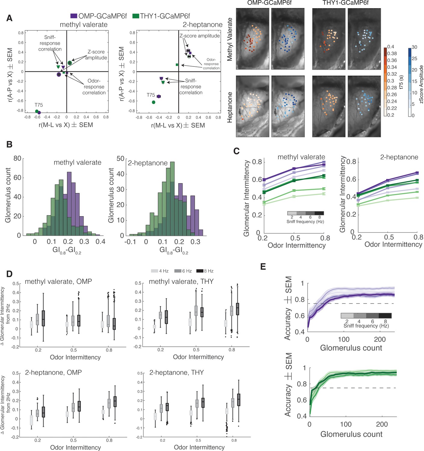
Additional quantification of the effect of sniff frequency on glomerular representation of intermittency.
For all graphs purple indicates olfactory sensory neurons (OSNs) (OMP-GCaMP6f) and green indicates mitral and tufted (M/T) cells (THY1-GCaMP6f). (A) Spatial maps of z-scored response amplitude (open circles) and odor-response correlation (diamonds) as well as spatiotemporal map (T75, filled circles) for methyl valerate (OMP, [M-L,A-P]: μz-score amplitude=[–0.16,–0.06], μodor-response corr=[–0.01,–0.02], μT75r=[–0.56,–0.85]; THY, [M-L,A-P]: μz-score amplitude=[0.06,0.17], μodor-response corr=[–0.06,–0.02], μT75r=[–0.61,–0.82]), left, and 2-heptanone (OMP, [M-L,A-P]: μz-score amplitude=[0.19,0.43], μodor-response corr=[0.23,0.38], μT75r=[–0.40,–0.51]; THY, [M-L,A-P]: μz-score amplitude=[0.21,0.31], μodor-response corr=[–0.03,0.14], μT75r=[–0.51,–0.63]), middle. Example spatial maps of t75 and z-score amplitude for OMP-GCaMP6f and THY1-GCaMP6f animals when presented with methyl valerate or heptanone, right. (B) Histogram of the change in glomerular intermittency (GI) from odor intermittency 0.2 to odor intermittency 0.8 based on the linear regression fit of GI vs odor intermittency per glomerulus. (C) Average GI as a function of odor intermittency for sniff frequencies of 2–8 Hz (light to dark shades). (D) GInHz-GI2Hz per glomerulus for each intermittency value for methyl valerate, top and 2-heptanone, bottom. (E) Linear classifier performance (accuracy) over 240 glomeruli when trained on trials of four different sniff frequencies (2, 4, 6, 8 Hz) when presented with methyl valerate. 60 iterations (20 times threefold) per classifier. OMP: exponential plateau fit, 2 Hz: Y=0.91–(0.34)*(e–0.03x), r2=0.55; 8 Hz: Y=0.86–(0.32)*(e–0.03x), r2=0.42. THY: exponential plateau fit, 2 Hz: Y=0.92–(0.5)*(e–0.05x), r2=0.66; 8 Hz: Y=0.93–(0.38)*(e–0.04x), r2=0.61.
Figure 6—figure supplement 2
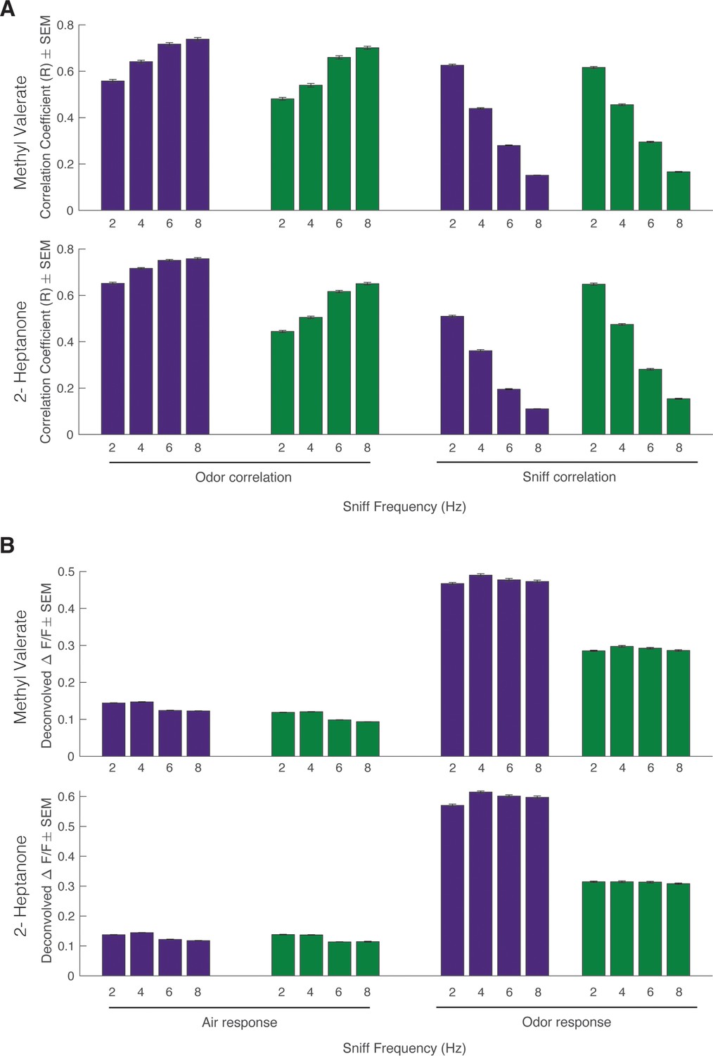
Effect of sniff frequency on odor correlation, sniff correlation, air response, and odor response.
For all graphs purple indicates olfactory sensory neurons (OSNs) (OMP-GCaMP6f) and green indicates mitral and tufted (M/T) cells (THY1-GCaMP6f). (A) Top: Methyl valerate. Bottom: 2-Heptanone. Left: Average maximum cross-correlation between glomerular response and photoionization detector (PID) reading across sniff frequencies (Spearman correlation, p<0.0001). Right: Average maximum cross-correlation between glomerular response and pressure sensor reading (sniff measurement) across sniff frequencies (Spearman correlation, p<0.0001). (B) Top: Methyl valerate. Bottom: 2-Heptanone. Left: Average glomerular deconvolved ΔF/F prior to odor presentation (Spearman correlation, p<0.0001). Right: Average glomerular deconvolved ΔF/F during odor presentation (Spearman correlation, p>0.05) (methyl valerate: OMP n=367 glomeruli, 7 mice; THY n=294 glomeruli, 6 mice; heptanone: OMP n=241 glomeruli, 6 mice; THY n=271 glomeruli, 6 mice; n=45 trials per sniff frequency, total n=180 trials).
Figure 7
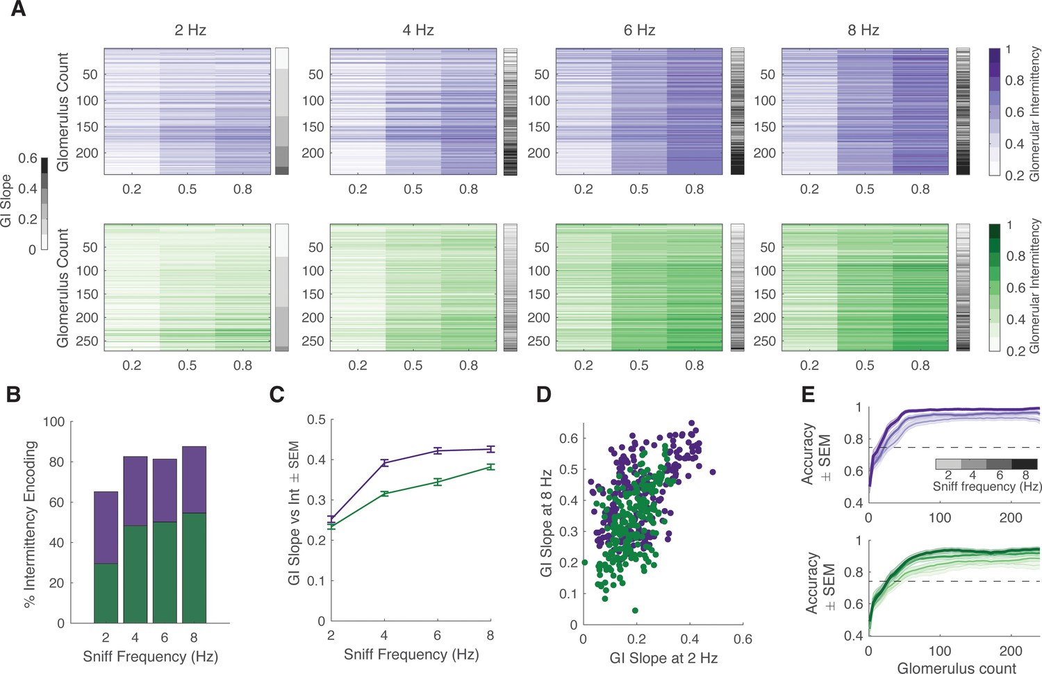
Effect of sniff frequency on glomerular representation of intermittency (2-heptanone).
For all graphs purple indicates olfactory sensory neurons (OSNs) (OMP-GCaMP6f) and green indicates mitral and tufted (M/T) cells (THY1-GCaMP6f). (A) Heatmap of glomerular intermittency across trials of 0.2, 0.5, and 0.8 odor intermittency values (colored heatmaps). Glomeruli are sorted based on their glomerular intermittency (GI) slope at 2 Hz. Gray bars next to heatmaps indicate the GI slope of each individual glomerulus. (B) % of intermittency encoding cells across sniff frequencies (OMP n=241 glomeruli, 6 mice; THY n=271 glomeruli, 6 mice). (C) GI slope as a function of sniff frequency. (D) GI slope at 8 Hz as a function of GI slope at 2 Hz. (E) Linear classifier performance (accuracy) over 240 glomeruli when trained on trials of four different sniff frequencies (2, 4, 6, 8 Hz). 60 iterations (20 times threefold) per classifier. Exponential plateau fit, OMP: 2 Hz: plateau = 0.95, Y=0.95–(0.44)*(e–0.04x), r2=0.67; 8 Hz: plateau = 0.98, Y=0.98–(0.37)*(e–0.04x), r2=0.7; THY: 2 Hz: plateau = 0.85, Y=0.85–(0.4)*(e–0.03x), r2=0.54; 8 Hz: plateau = 0.94, Y=0.94–(0.4)*(e–0.04x), r2=0.64.
Additional files
Download links
A two-part list of links to download the article, or parts of the article, in various formats.
Downloads (link to download the article as PDF)
Open citations (links to open the citations from this article in various online reference manager services)
Cite this article (links to download the citations from this article in formats compatible with various reference manager tools)
Behavioral discrimination and olfactory bulb encoding of odor plume intermittency
eLife 13:e85303.
https://doi.org/10.7554/eLife.85303


