Resting-state fMRI signals contain spectral signatures of local hemodynamic response timing
- Department of Biomedical Engineering, Boston University, United States
- Athinoula A. Martinos Center for Biomedical Imaging, Massachusetts General Hospital, United States
- Department of Radiology, Harvard Medical School, United States
- Graduate Program for Neuroscience, Boston University, United States
- Institute for Medical Engineering and Science, Massachusetts Institute of Technology, United States
- Department of Electrical Engineering and Computer Science, Massachusetts Institute of Technology, United States
Figures
Figure 1 with 2 supplements

Simulations show that the temporal properties of the hemodynamic response function affect the frequency spectrum of the BOLD signal.
(A) We generated a simulated BOLD response to determine the response amplitude of each HRF to each neural frequency. By convolving a given HRF with an oscillating stimulus, and sweeping across a range of frequencies, we generated a frequency spectrum of the simulated BOLD responses. This simulation was repeated using HRFs with varying temporal properties, to compare the frequency spectrum of simulated BOLD responses with faster or slower hemodynamic responses. (B) We generated a range of HRFs with physiologically plausible timings and amplitudes (Siero et al., 2011). (C) We found that temporal properties of the HRF had noticeable effects on the simulated spectra, particularly under 0.2 Hz.
Figure 1—figure supplement 1

Simulation results are robust to changes in HRF amplitude and 1 /f decay of stimulus amplitude.
(A) We normalized each HRF to its respective peak amplitude to examine effect on frequency spectra. (B) The differences in spectral content of the BOLD signal are not simply due to the amplitude of each HRF but rather a signature of the temporal dynamics of the HRF, as the slope differences persist when normalizing for amplitude, with slower HRFs generating steeper frequency responses. (C) Plot showing the magnitudes of the neural waveform at each frequency and their 1 /f decay. (D) Physiologically relevant HRFs used in simulations. (E) Temporal properties of HRF noticeably affect the slope of the simulated spectra even when oscillation amplitudes decay with 1 /f pattern, demonstrating that distinct slopes are expected for distinct HRFs regardless of the specific neural signal amplitude.
Figure 1—figure supplement 2

Impact of varying either TTP or FWHM on the power spectrum of simulated BOLD signals.
(A) We generated a set of 6 HRFs with a fixed TTP of 6 s, variable FWHMs ranging from 2 to 6 s, and the same amplitude. (B) Changing the FWHM of the HRF has noticeable effects on the simulated frequency spectra. (C) The slope of the frequency spectrum under 0.2 Hz was positively correlated with the FWHM. (D) We generated another set of 6 HRFs with variable TTPs ranging from 2 to 6 s, a fixed FWHM of 3 s, and the same amplitude. (E) Changing the TTP of the HRF has a smaller effect on the simulated frequency spectra. (F) The slope of the frequency spectrum under 0.2 Hz was positively correlated with the TTP.
Figure 2

Experimental design: oscillating visual stimuli identify fast- and slow-responding voxels in V1.
(A) Subjects viewed a flickering checkerboard with oscillating luminance contrast to drive neural oscillations in V1. Some voxels showed a faster response to the visual stimulus and other showed a slower response, with a noticeable difference in the temporal dynamics of the mean response in these groups. Shading represents standard error. (B) Example of a functional localizer in one subject with the white lines denoting the outline of the primary visual cortex (V1) based on anatomical segmentation. One visual stimulus run was used as a functional localizer to identify stimulus-driven voxels in V1. (C) For all stimulus-driven voxels in V1, the phase of the response to the visual stimulus was calculated from the average of the visual stimulus runs not used as the functional localizer, corresponding to the local hemodynamic delay. (D) We defined groups of ‘fast’ and ‘slow’ voxels using a Gaussian fit to the histogram of phases. Histogram shows example from one representative subject. (E) Example map of fast and slow voxels generated for a single subject. (F) Frequency spectrum of a representative slow and fast voxel’s resting-state signal, showing a difference in power drop off across frequencies, with a steeper slope for the slower voxel.
Figure 3 with 3 supplements

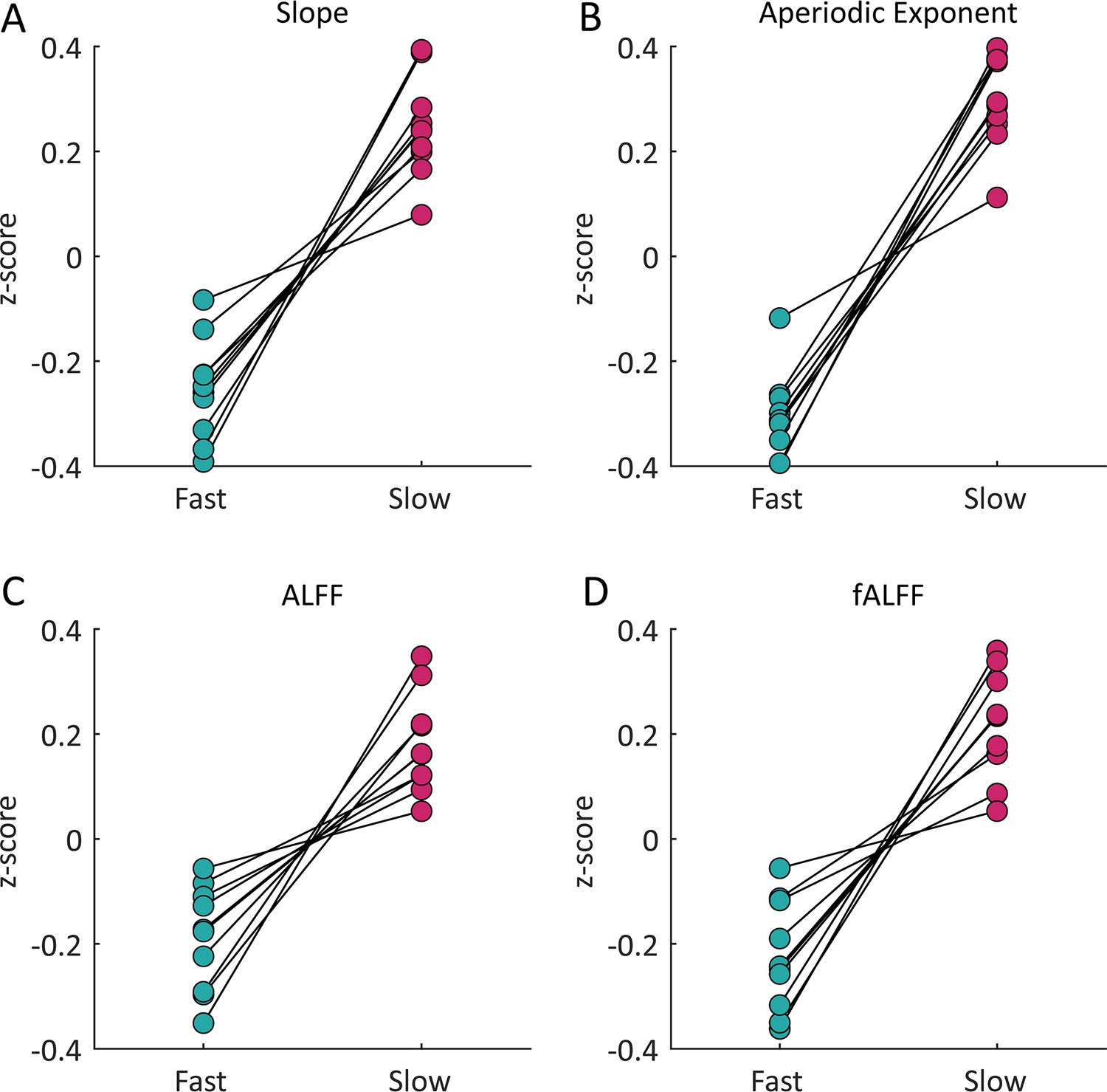
Features of the resting-state spectrum differed between fast and slow voxels in each subject.
For each subject, we calculated four features of the resting-state frequency spectrum and compared the values between the task-defined fast and slow voxels using a Wilcoxon rank sum test. For the (A) slope, using a linear fit of frequency spectrum under 0.2 Hz, 15/15 subjects showed significant differences; (B) exponent of an aperiodic 1 /f fit under 0.5 Hz, 14/15 subjects showed significant differences; (C) amplitude of low frequency fluctuations (ALFF), 11/15 subjects showed significant differences; and (D) fractional ALFF, 13/15 subjects showed significant differences. Black lines indicate a significant difference in a given subject (Wilcoxon rank-sum test, p<0.05) and red lines indicate a non-significant difference.
Figure 3—figure supplement 1
The same pattern of frequency content for fast and slow voxels replicated in an independent dataset acquired at 3T.
Based on our simulations and data collected at 7 Tesla we expected that for each spectral feature the slow voxels will have higher values than the fast voxels. In an independent replication dataset at 3T, for each spectral feature all 10 subjects followed this expected pattern further demonstrating the robustness of this phenomenon. For both the (A) slope of a linear fit of the frequency spectrum under 0.2 Hz and (B) exponent of an aperiodic 1 /f fit under 0.5 Hz 9/10 subjects showed significant differences at the individual level. For both the (C) ALFF and (D) fALFF 8/10 subjects showed significant differences at the individual level. All differences were significant (p<0.05) at the group level.
Figure 3—figure supplement 2

There is no consistent pattern of relationship between fast and slow voxels’ estimated noise floor of the frequency spectrum.
We did not observe a consistent effect on the noise floor between fast and slow voxels, with no significant difference at the group level.
Figure 3—figure supplement 3

Example subjects showing significant (p<0.05) correlations between each spectral feature and phase on a voxel-wise basis.
Each point represents a single voxel, red-line shows linear fit. p-values are from a linear hypothesis test on the model coefficients. (A) Example subject showing significant, positive correlations between each spectral feature and the magnitude of the phase. (B) A second example subject also showing a significant, positive correlation between each spectral feature and the magnitude of the phase.
Figure 4 with 1 supplement

The coupling of response timing and resting-state spectral content is maintained in the LGN.
(A) Example LGN localizer in one subject showing uncorrected z-statistic in the localizer run within the anatomical mask of LGN defined by the white outline. (B) Average time series of fast and slow V1 voxels compared to LGN voxels for an example subject. LGN displayed a fast visually-driven response, leading even the earliest cortical voxels. Time series are smoothed for display using a 10-point moving average. Shading represents standard error. (C–F) For each subject we calculated the four resting-state spectral features for the LGN and compared them to the fast and slow voxels in V1. For the (C) slope, 15/15 subjects showed significant differences between fast vs. LGN and slow vs. LGN; (D) exponent of an aperiodic 1 /f fit, 15/15 subjects showed significant differences between fast-LGN and slow-LGN; (E) ALFF, 5/15 subjects showed significant differences between fast vs. LGN and 7/15 between slow vs. LGN; and (F) fALFF, 15/15 subjects showed significant differences between fast-LGN and between slow-LGN. Black lines indicate a significant difference (Wilcoxon rank-sum test, p<0.05) and red lines indicate a non-significant difference.
Figure 4—figure supplement 1

Accounting for thermal noise does not significantly change the estimated slope of the frequency spectrum under 0.2 Hz in V1 or LGN voxels.
(A) Spectra of example LGN voxel demonstrating the method for accounting for the noise floor in the slope of the linear fit. The original linear fit and the linear fit with the noise floor produce similar results. (B) Average magnitude of slopes before and after fitting the noise floor in fast and slow cortical voxels as well as LGN voxels with error bars showing SEM. The within group averages did not significantly change when fitting for the noise floor versus not.
Figure 5 with 1 supplement

Breath hold vascular latencies yield less robust characterization of task-driven hemodynamic response lags.
(A) Plot of one subject’s average BOLD response to the breath hold task in fast (teal) and slow (pink) cortical voxels as well as LGN voxels (yellow). The shaded areas are the standard error across voxels of that group. Colored arrows denote the peak of the response to the breath hold. The LGN time series peaks slightly earlier than the fast cortical voxels and both the LGN and fast cortical voxels peak well before the slow cortical voxels. This sequence of activation matches what is expected based on the hemodynamic lags across these structures. (B) Plot of one subject’s average BOLD response to the breath hold task where the order of activation is not as expected. While the slow cortical voxels reached their peak last, the fast cortical voxels peaked before LGN voxel, meaning that the breath hold would not accurately predict latency in this subject. (C) Comparison of the average breath hold latency in fast, slow, and LGN voxels in all subjects. For 9/15 subjects, the average latency of the fast cortical voxels was less than the slow cortical voxels, as expected, and 7 of these 9 had a significant difference. For only 2/15 subjects, the average latency of the LGN voxels was less than fast voxels, as expected, but only 1 of these 2 had a statistically significant difference. For 4/15 subjects, the average latency of slow cortical voxels was larger than LGN voxels, and 1 of these 4 had a statistically significant difference. (Wilcoxon rank-sum test, p<0.05).
Figure 5—figure supplement 1

Subject motion during the breath hold task was significantly worse than the visual stimulus task.
Boxplot shows the average framewise displacement per task condition across subjects. There was significantly more motion during the breath-hold task than during the visual task (Wilcoxon rank-sum test, p=0.01), but no significant difference in motion between the visual stimulus and resting-state runs (p=0.431). There was a trend towards more motion in the breath hold runs compared to the resting-state runs (p=0.051).
Figure 6 with 1 supplement

Average classification accuracy of SVM classifier trained using different features.
The classification accuracies reported are the average validation accuracy across 1000 bootstraps. The black markers indicate the models trained using resting-state spectral features from all subjects combined into one model; the colored markers show results from individual subjects (n=15). Both models trained using features of the resting-state spectrum performed significantly better than the model trained using the breath hold latencies; however, there was no significant difference in performance between the two models trained using information from the resting-state spectrum (=0.283). All classifiers perform significantly above chance (33%). *** p<0.0005 (Wilcoxon rank-sum test).
Figure 6—figure supplement 1

Classification accuracies of SVM classifier when requiring that training and test voxels be physically separated.
We trained a second model to test whether we could predict early and late voxels when training and test voxels were in distinct locations. All validation accuracies reported for the 80–20 test-train split are the average validation accuracy across 1000 bootstraps. The validation accuracies reported for the LH-RH test-train split are from training the model using one hemisphere and validating the model on the other hemisphere. (A) Each colored marker shows results from an individual subject (N=15). For some subjects, the validation accuracy decreased when using a LH-RH split while others increased. All classifiers performed well above chance (33%). (B) The model trained using features from all subjects had a higher validation accuracy when using a LH-RH split compared to the random 80–20 split, suggesting improved generalization across subjects when training on spatially separated voxels.
Additional files
-
MDAR checklist
- https://cdn.elifesciences.org/articles/86453/elife-86453-mdarchecklist1-v2.docx
-
Supplementary file 1
Subject-wise p-values of Wilcoxon rank-sum test comparing each spectral feature in fast and slow voxels.
- https://cdn.elifesciences.org/articles/86453/elife-86453-supp1-v2.docx
-
Supplementary file 2
Subject-wise average SVM classification accuracy with confidence intervals.
- https://cdn.elifesciences.org/articles/86453/elife-86453-supp2-v2.docx
-
Supplementary file 3
Subject-wise results from fit of linear model relating each spectral feature with phase.
- https://cdn.elifesciences.org/articles/86453/elife-86453-supp3-v2.docx
-
Supplementary file 4
Subject-wise performance of regression model to predict specific response timing from spectral features.
- https://cdn.elifesciences.org/articles/86453/elife-86453-supp4-v2.docx
-
Supplementary file 5
Parameters of simulated HRFs.
- https://cdn.elifesciences.org/articles/86453/elife-86453-supp5-v2.docx
Download links
A two-part list of links to download the article, or parts of the article, in various formats.
Downloads (link to download the article as PDF)
Open citations (links to open the citations from this article in various online reference manager services)
Cite this article (links to download the citations from this article in formats compatible with various reference manager tools)
Resting-state fMRI signals contain spectral signatures of local hemodynamic response timing
eLife 12:e86453.
https://doi.org/10.7554/eLife.86453


