Repeatability of adaptation in sunflowers reveals that genomic regions harbouring inversions also drive adaptation in species lacking an inversion
- Department of Biological Sciences, University of Calgary, Canada
- Department of Botany, University of British Columbia, Canada
- Michael Smith Laboratories, University of British Columbia, Canada
- Irving K. Barber Faculty of Science, University of British Columbia Okanagan, Canada
- Department of Biology, University of Victoria, Canada
Figures
Figure 1
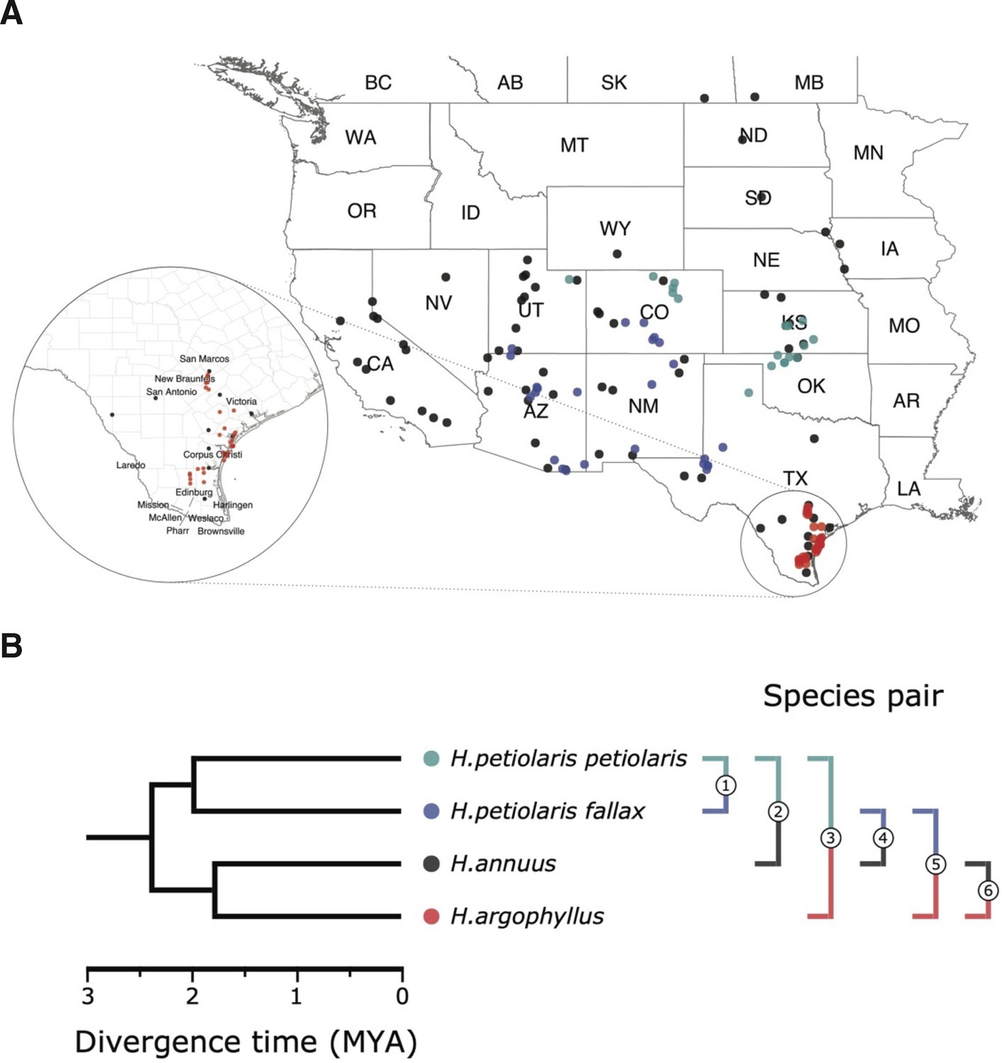
Sampling sites and phylogenetic relationship among surveyed species.
(A) Sampling locations of wild sunflower populations studied in this study, and (B) phylogenetic relationship of the four (sub-)species. Numbered brackets represent the six pairwise comparisons performed in this study.
Figure 2
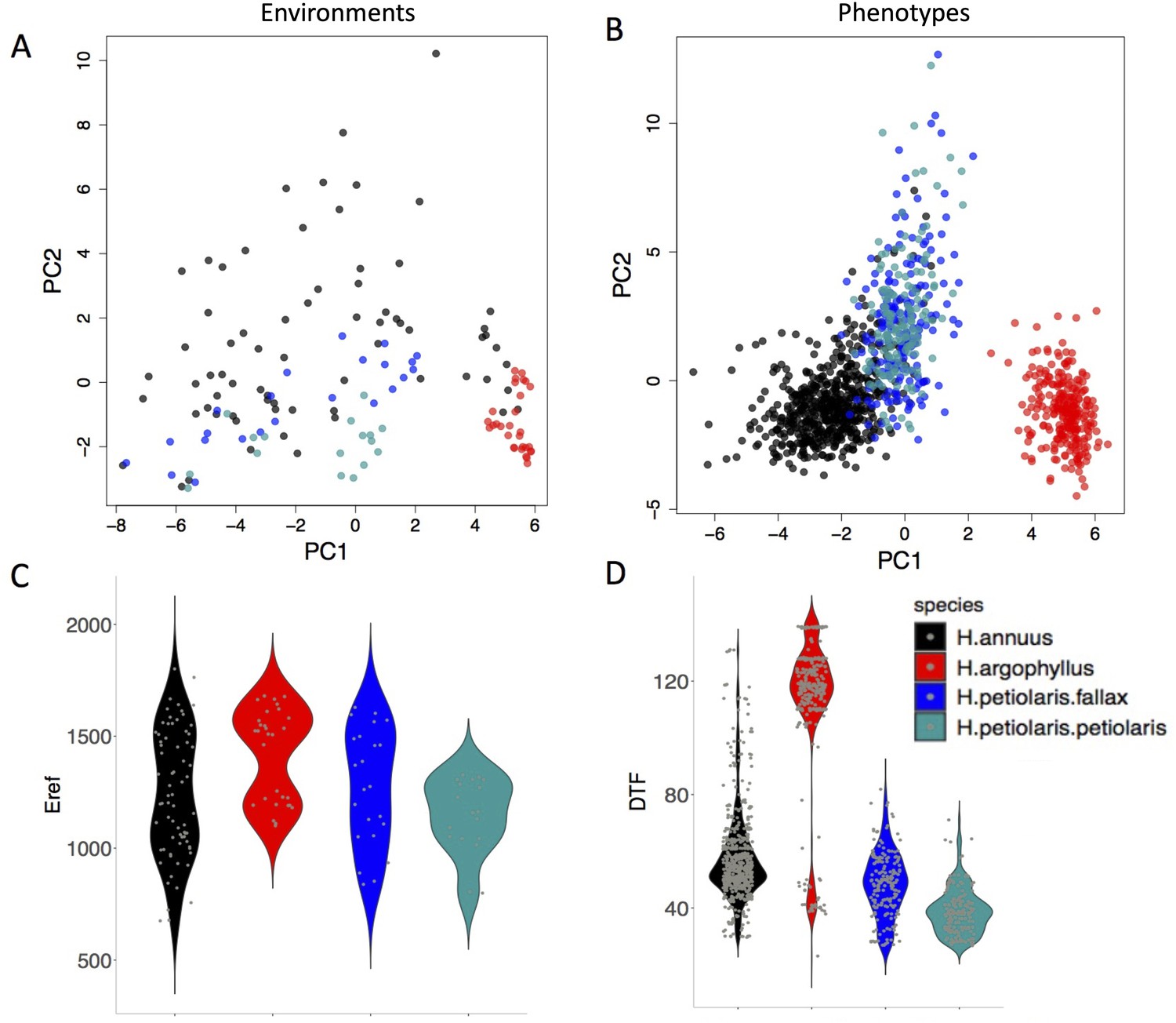
The range of environmental and phenotypic variation in the studied species.
Variation in environment (A) and phenotype (B) for the studied species, along the two largest axes of a principal component analysis (PCA). Violin plots show two examples of variation in environment (Hargreaves reference evapotranspiration index; Eref) and phenotype (Days to Flower; DTF) within and among the taxa (C, D).
Figure 3
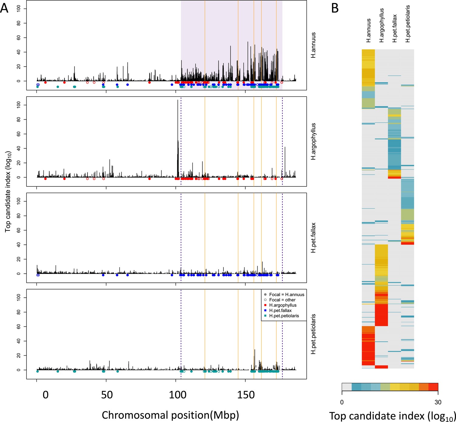
Signatures of association for number of frost-free days (NFFD) in the four taxa on chromosome 15 (A) and genome-wide (B).
Panel (A) shows windows of repeated association (WRAs; coloured bars) for comparisons between the focal species, H. annuus, and each of the other three taxa, with the haploblocks in H. annuus shaded in violet and the regions with significant PicMin hits as vertical orange lines. Panel (B) shows the value of the top candidate index for each of the 1000 windows with the strongest signatures of association in at least one species (approximately top 2% of genome-wide windows). Rows are ordered using hierarchical clustering to group windows with similar patterns across multiple species, illustrating the extent of overlap/non-overlap in the windows with strongest signatures in each species (i.e. position in the figure does not reflect chromosomal position).
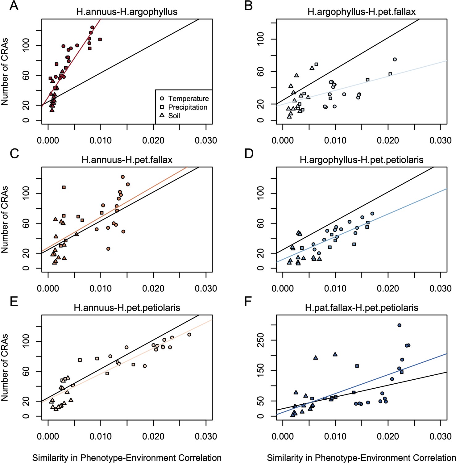
Figure 4
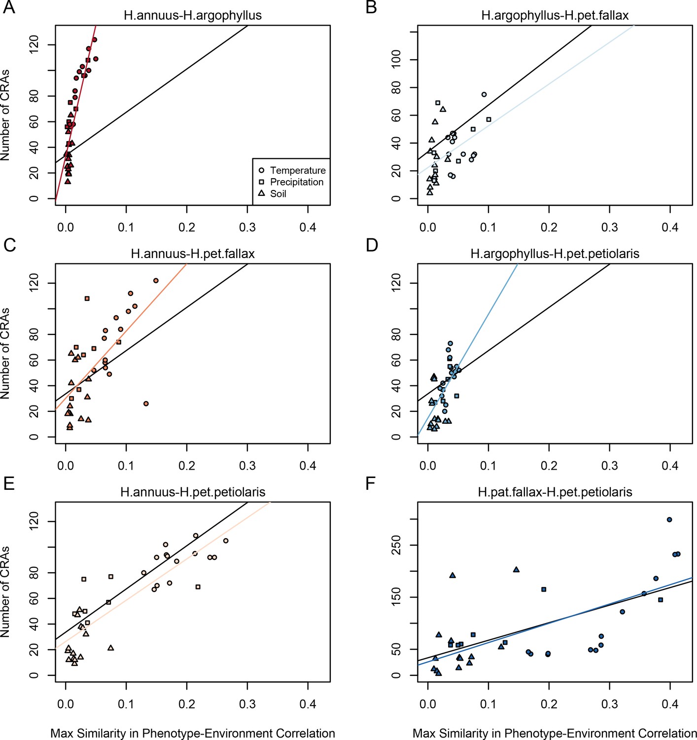
Relationship between maximum similarity in phenotype–environment correlation (SIPEC) and number of clusters of repeated association (CRAs).
SIPEC was calculated for each phenotypic principal component analysis (PCA) axis, with the maximum taken across the axes that cumulatively explain 95% of the phenotypic variance for each environment. Each panel (A-F) shows a comparison between a pair of species indicated above, and includes both a linear model fit to the data within the panel (coloured lines), and a linear model fit to all data simultaneously (black lines) for comparison. Note that because environmental variables are correlated, these points are not independent and therefore represent a source of pseudoreplication, preventing formal statistical tests of this relationship.
Figure 5
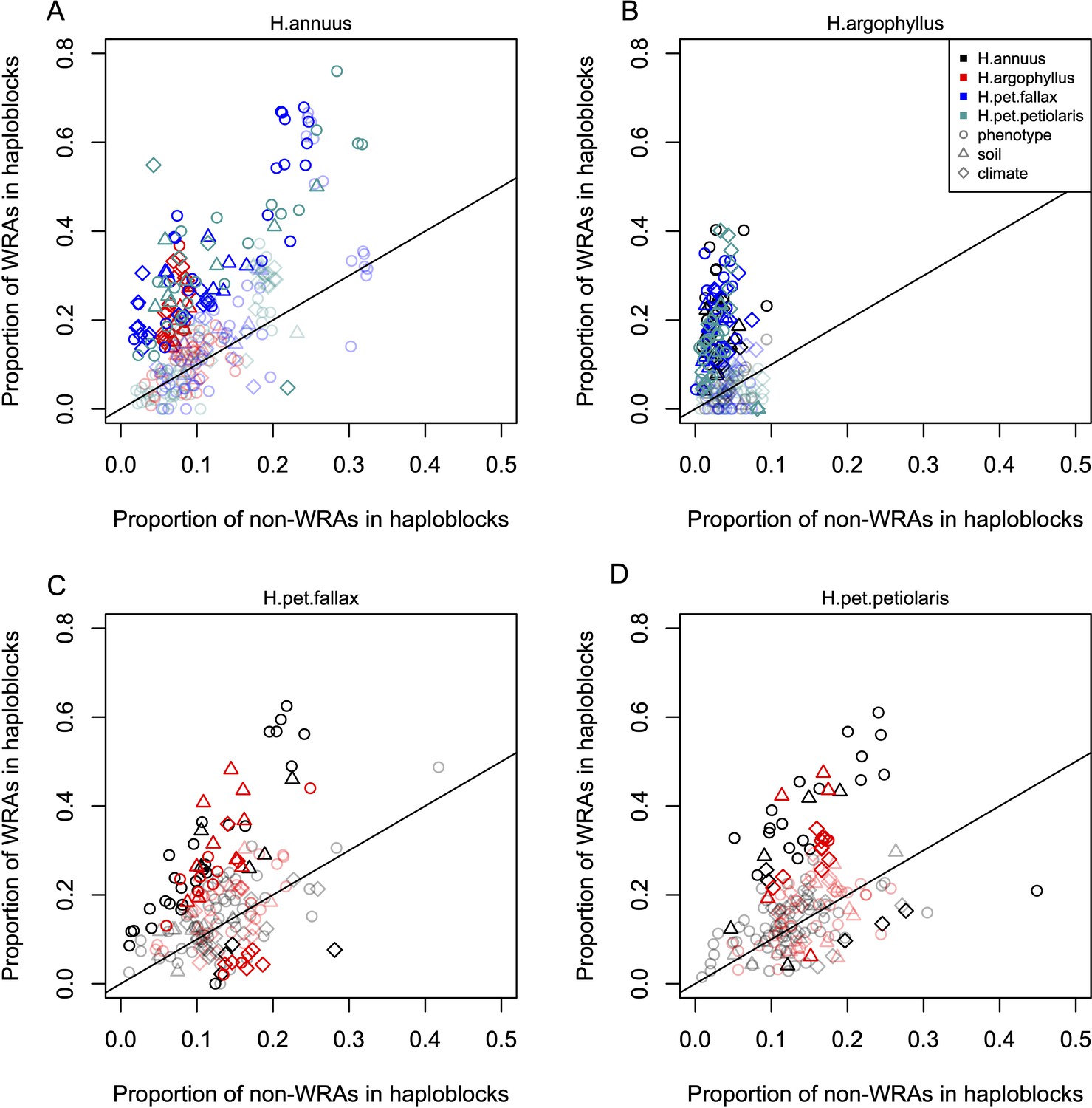
Enrichment of signatures of repeated association within genomic regions harbouring a haploblock in one of the two compared lineages.
Each panel shows the proportion of top candidate windows that fall within haploblocks for windows with significant signatures of repeated association by the null-W test (windows of repeated association [WRAs]) vs. those with non-significant signatures (non-WRAs), with a different focal species plotted in each panel (A-D). Comparisons of H. petiolaris petiolaris vs. H. petiolaris fallax are omitted as they share segregating haploblocks. Each point corresponds to the results for a single phenotype or environment, with dark shading used for cases where the deviation from random for the contingency table is significant by a permutation test (p<0.05), and lighter shading indicating a non-significant result. Note that because many environmental variables and phenotypes are correlated with each other, these points are not independent and therefore represent a source of pseudoreplication, preventing formal statistical tests of the overall relationship within each panel.
Appendix 1—figure 1
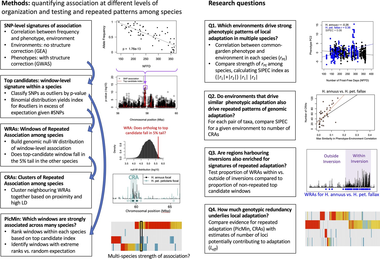
Schematic overview of methods and primary research questions.
Appendix 1—figure 2
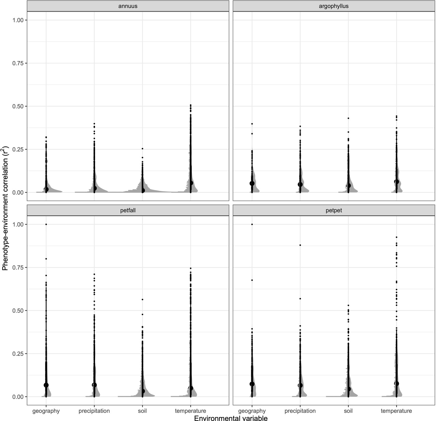
Strength of phenotype–environment correlations across all traits for four different types of environmental variables in each of the sunflower species and subspecies.
Black points show individual values, and grey points show binned density.
Appendix 1—figure 3
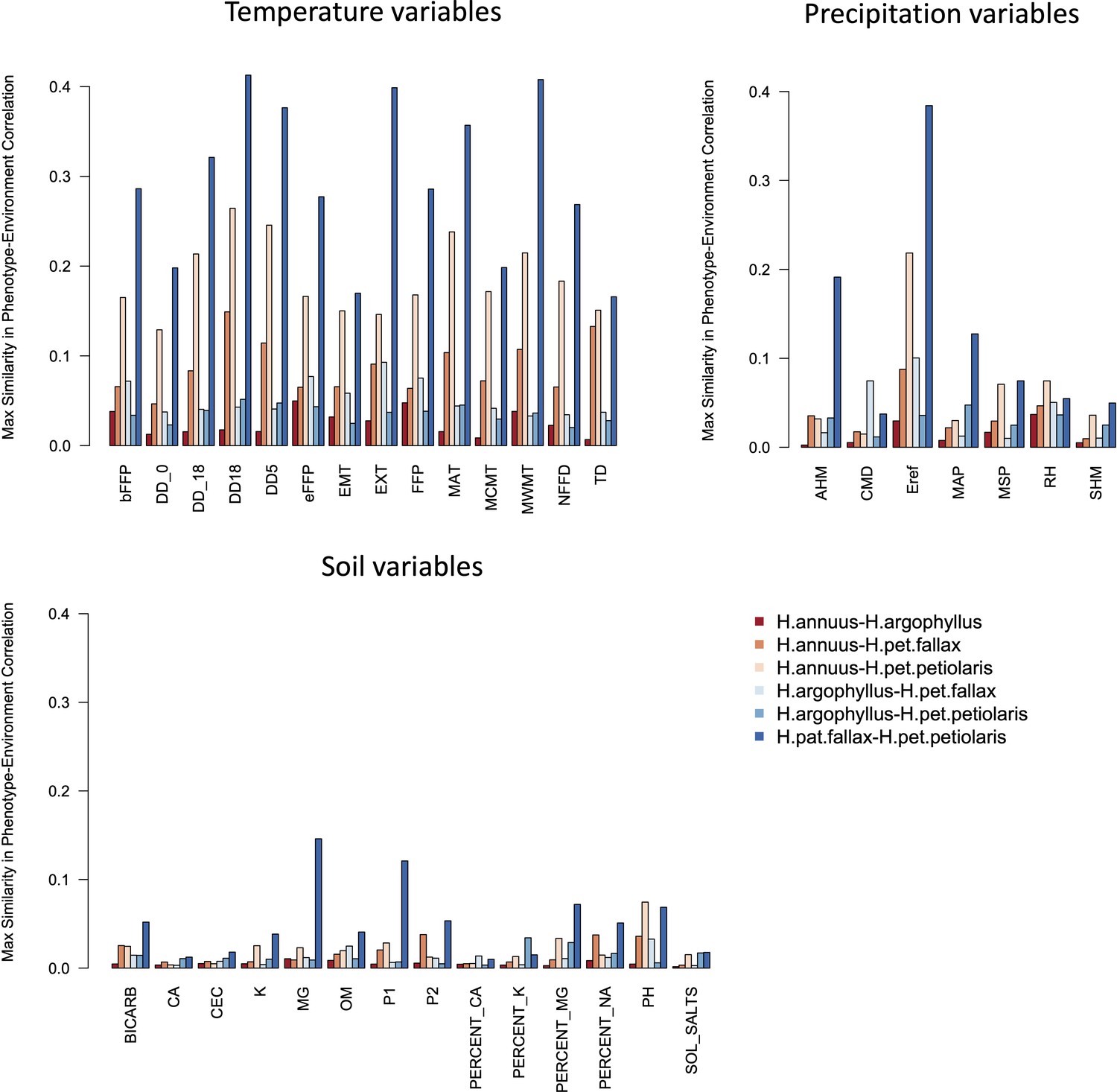
Maximum similarity in phenotype–environment correlation (SIPEC) for pairs of taxa, across soil-, temperature-, and precipitation-related environmental variables.
The maximum value of SIPEC for each environment is calculated across all phenotypic principal component analysis (PCA) axes that cumulatively explain 95% of the variance.
Appendix 1—figure 4
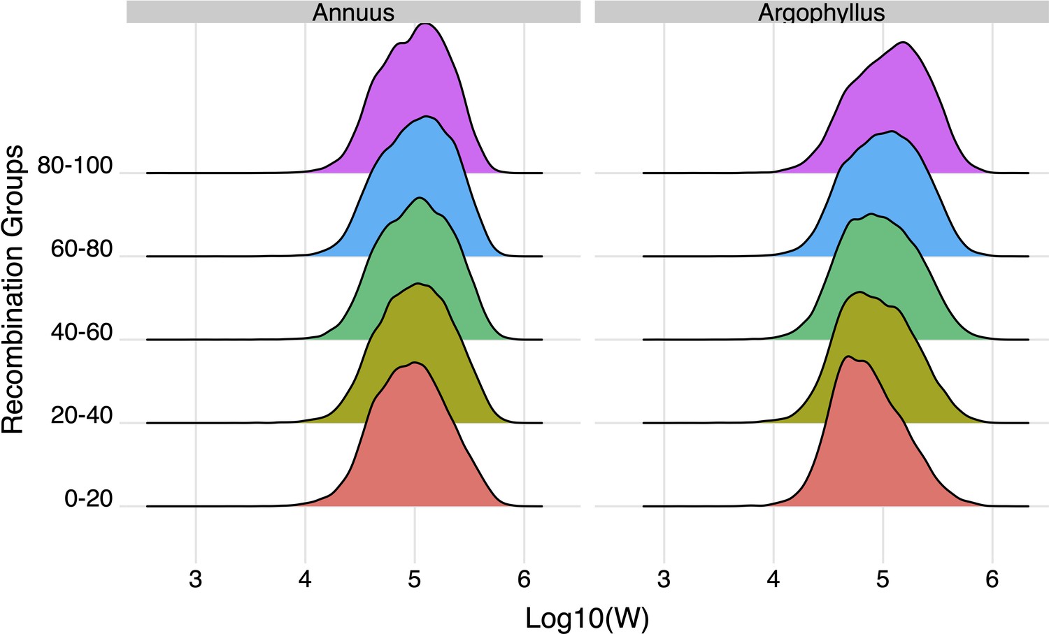
The effect of recombination rate on width of the null-W distribution for the number of frost-free days (NFFD) variable for Helianthus annuus and H. argophyllus.
Recombination bins represent the 0th–20th percentile, 20th–40th percentile, etc.
Appendix 1—figure 5
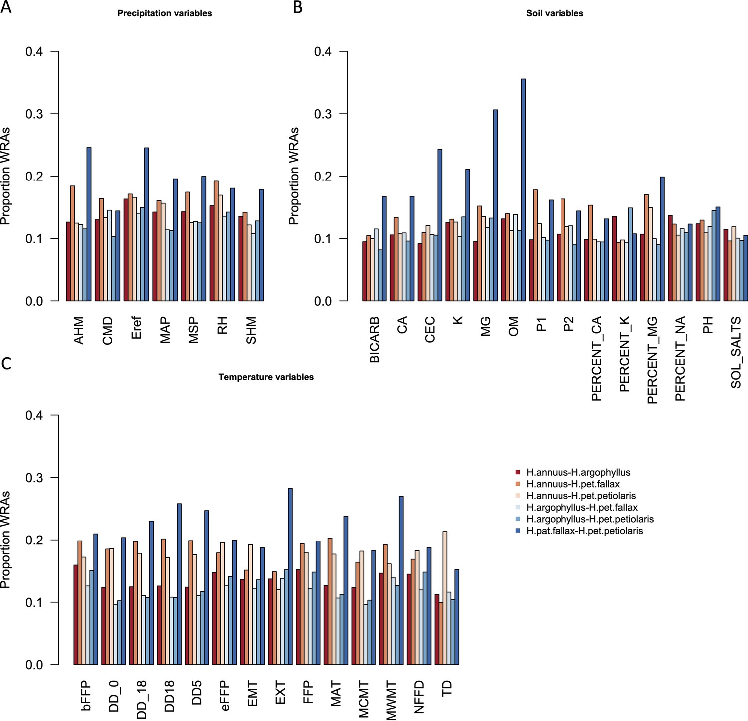
Proportion of top candidate windows that are significant hits under the null-W test (windows of repeated association), for pairs of taxa, across precipitation (A), soil (B), and temperature (C) environmental variables.
Appendix 1—figure 6
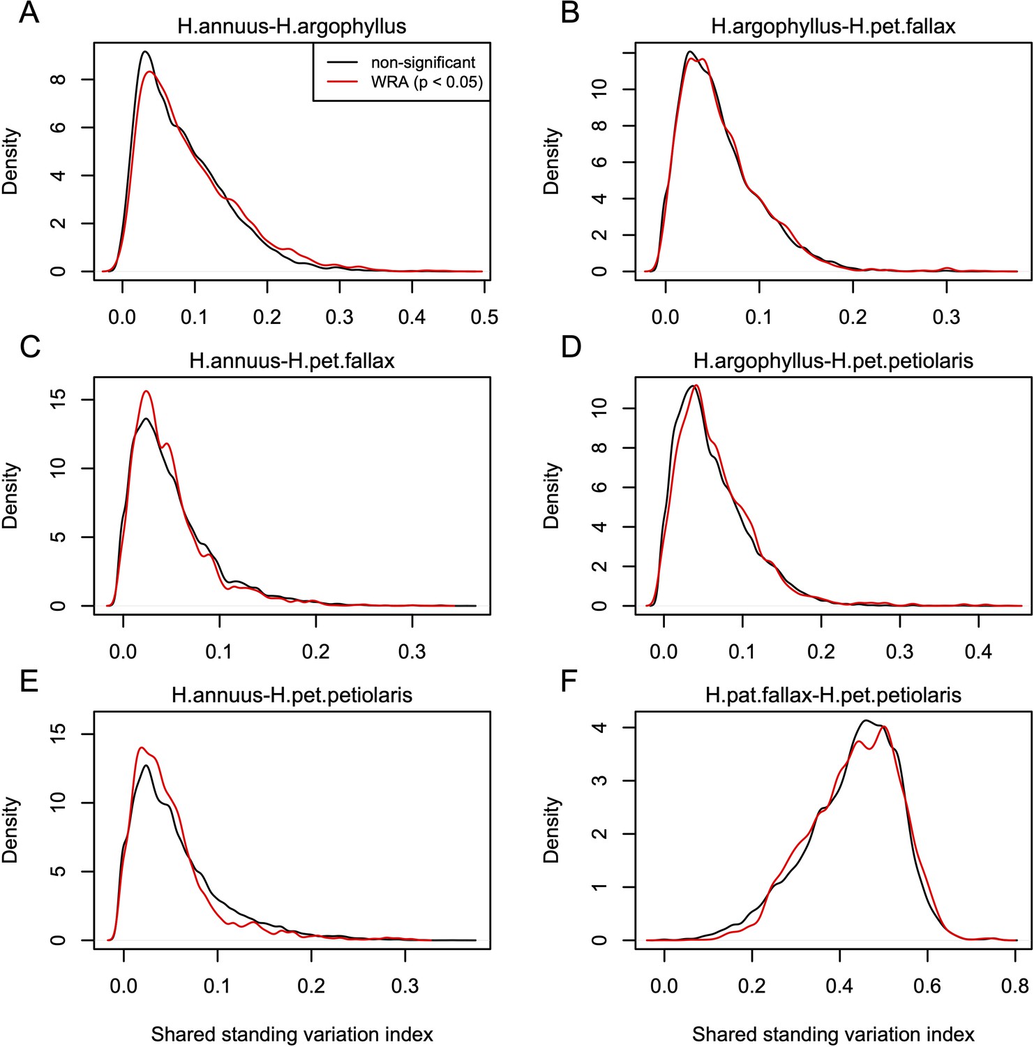
Index of shared standing variation for windows of repeated association (WRAs) vs. top candidates that were not significant under the null-W test.
The index of shared standing variation reflects the proportion of SNPs that are shared vs. non-shared among species and provides an indicator of the likely extent of introgression, which does not appear to differ substantially among the windows of the genome with significant (p<0.05; red lines) vs. non-significant (p>0.05; black lines) null-W test results. Panels A-F show the values for each of the six pairwise comparisons among species, as indicated above each panel.
Appendix 1—figure 7
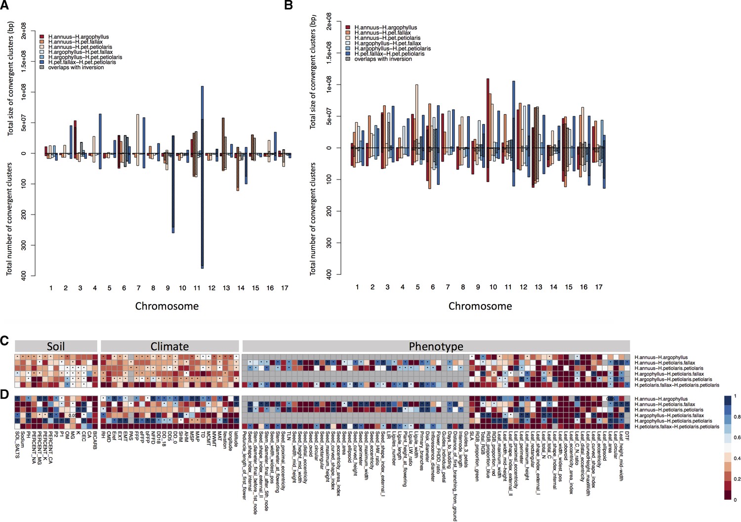
Number and size of clusters of repeated association (CRAs) and their overlap with haploblocks.
Total size and total number of CRAs detected among six studied pairs on each linkage group across all phenotypes by Genome-Wide Association (GWAS) (A), and Genotype-Environment Association (GEA) (B). Hatching areas indicate the total size and number of clusters residing within chromosomal rearrangements. Heat maps present proportion of CRAs by number (C) and size (D) per each phenotype variable and environment variable overlapping with chromosomal rearrangements. Stars in indicate overlaps between CRAs and haploblocks happen significantly different from chance (p-value ≤ 0.05). Grey cells in the heat maps indicate no data is available for that comparison and variable.
Appendix 1—figure 8
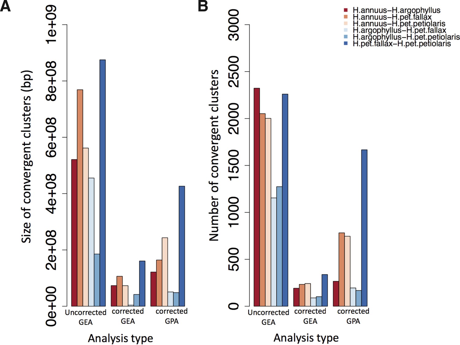
Total size and number of convergent clusters in different pairs for each analysis type.
The total size of convergent clusters (A) and total number of convergent clusters (B) identified among different pairs surveyed in the present study using association genetic approaches that corrected population structure versus those that did not correct across all environmental variables (GEA) and corrected GWAS.
Appendix 1—figure 9
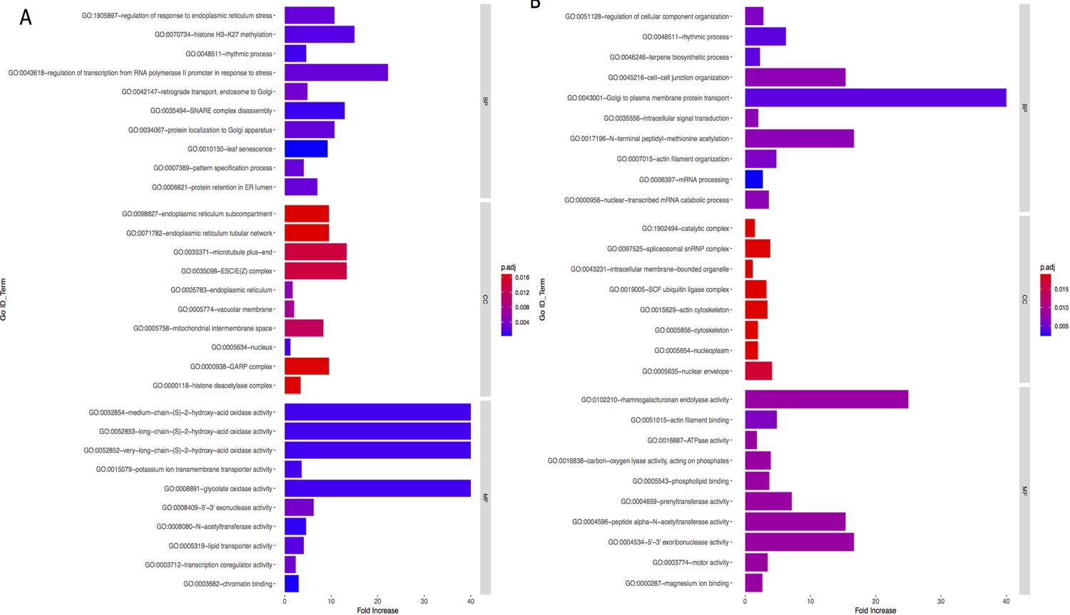
Bar graph of Gene Ontology (GO) enrichment analysis for phenotype (A) and precipitation-related variables (B).
Bar plot depicts the significant enriched GO terms within categories: biological process, cellular component, and molecular function. Y-axis represents the GO term, and the X-axis represents the enrichment significance, respectively.
Appendix 1—figure 10
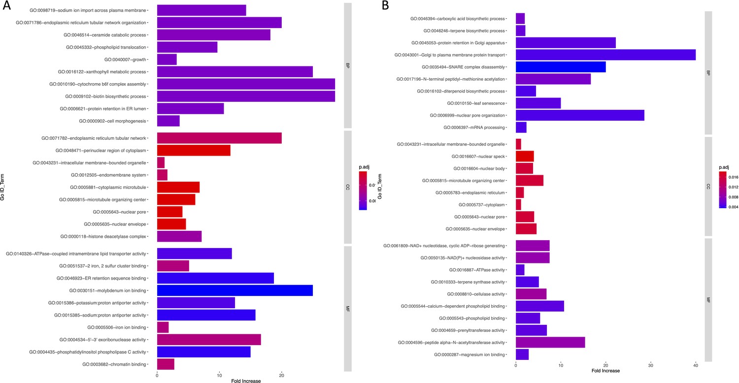
Bar graph of Gene Ontology (GO) enrichment analysis for soil (A) and temperature-related variables (B).
Bar plot depicts the significant enriched GO terms within categories: biological process, cellular component, and molecular function. Y-axis represents the GO term, and the X-axis represents the enrichment significance.
Appendix 1—figure 11
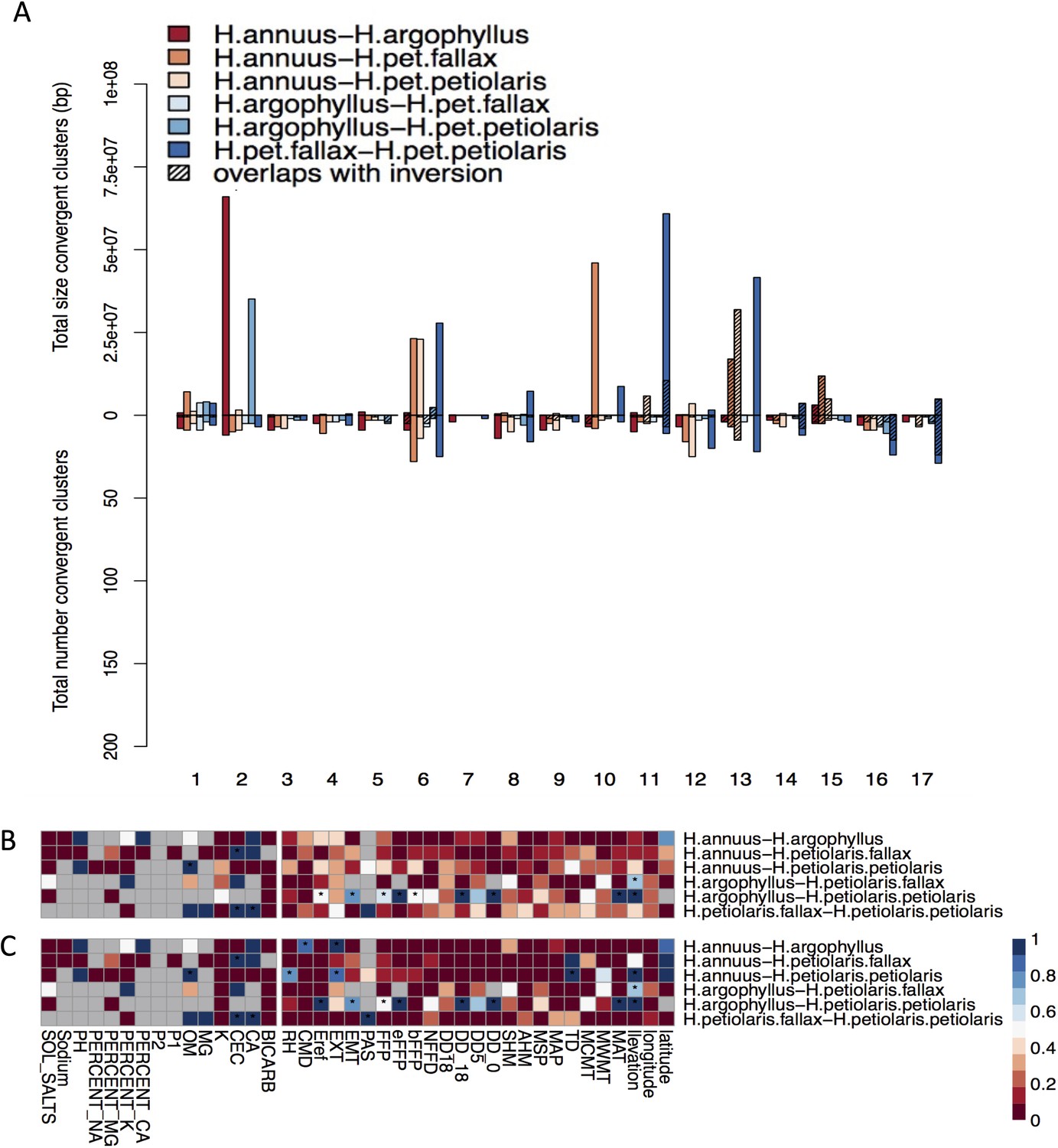
Effect of structure correction on number and size of clusters of repeated association (CRAs) and their overlaps with inversions.
Total size and total number of CRAs detected among six studied pairs on each linkage group across all environmental variables by corrected GEA (A). Hatching areas indicate the total size and number of clusters residing within haploblocks. Heat maps present proportion of CRAs overlapping with haploblocks by number (B) and size (C) for each phenotype and environmental variable (climate and soil). Stars indicate cases where observed overlaps between CRAs and haploblocks happen significantly more than expected by chance (p-value ≤ 0.05). Grey cells in the heat maps indicate no data is available for that comparison and variable.
Appendix 1—figure 12
Relationship between mean similarity in phenotype-environment correlation (SIPEC) and number of clusters of repeated association (CRAs).
SIPEC was calculated for each phenotypic principal component analysis (PCA) axis with the mean calculated across the axes that cumulatively explain 95% of the phenotypic variance for each environment. Each panel (A-F) shows a comparison between a pair of species indicated above, and includes both a linear model fit to the data within the panel (coloured lines), and a linear model fit to all data simultaneously (black lines) for comparison. Note that because environmental variables are correlated, these points are not independent and therefore represent a source of pseudoreplication, preventing formal statistical tests of this relationship.
Appendix 1—figure 13
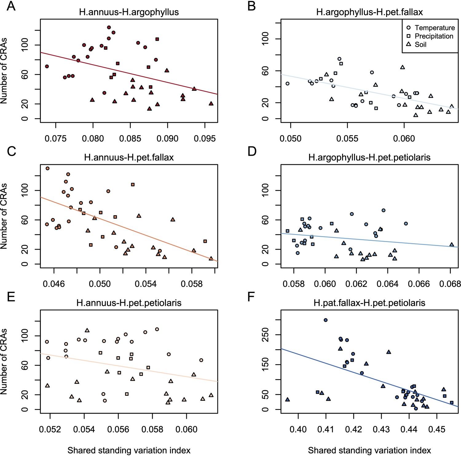
Relationship between index of shared standing variation and number of clusters of repeated association (CRAs).
Panels A-F show the values for each of the six pairwise comparisons among species, as indicated above each panel, with lines showing linear model fits for data within each panel.
Appendix 1—figure 14
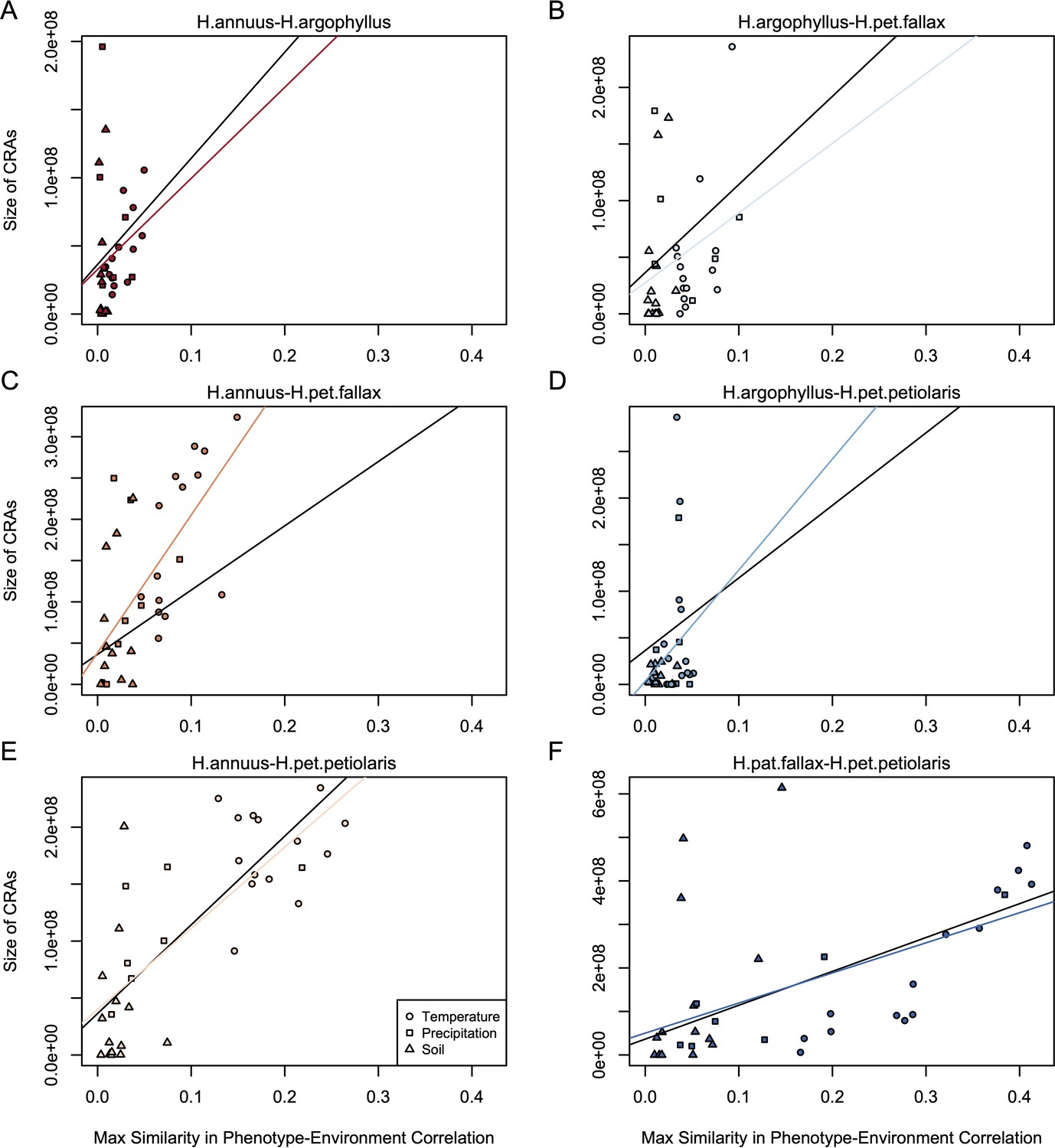
Relationship between mean similarity in phenotype–environment correlation (SIPEC) and size of clusters of repeated association (CRAs).
SIPEC was calculated for each phenotypic principal component analysis (PCA) axis with the mean calculated across the axes that cumulatively explain 95% of the phenotypic variance for each environment. Each panel (A-F) shows a comparison between a pair of species indicated above, and includes both a linear model fit to the data within the panel (coloured lines), and a linear model fit to all data simultaneously (black lines) for comparison. Note that because environmental variables are correlated, these points are not independent and therefore represent a source of pseudoreplication, preventing formal statistical tests of this relationship.
Appendix 1—figure 15
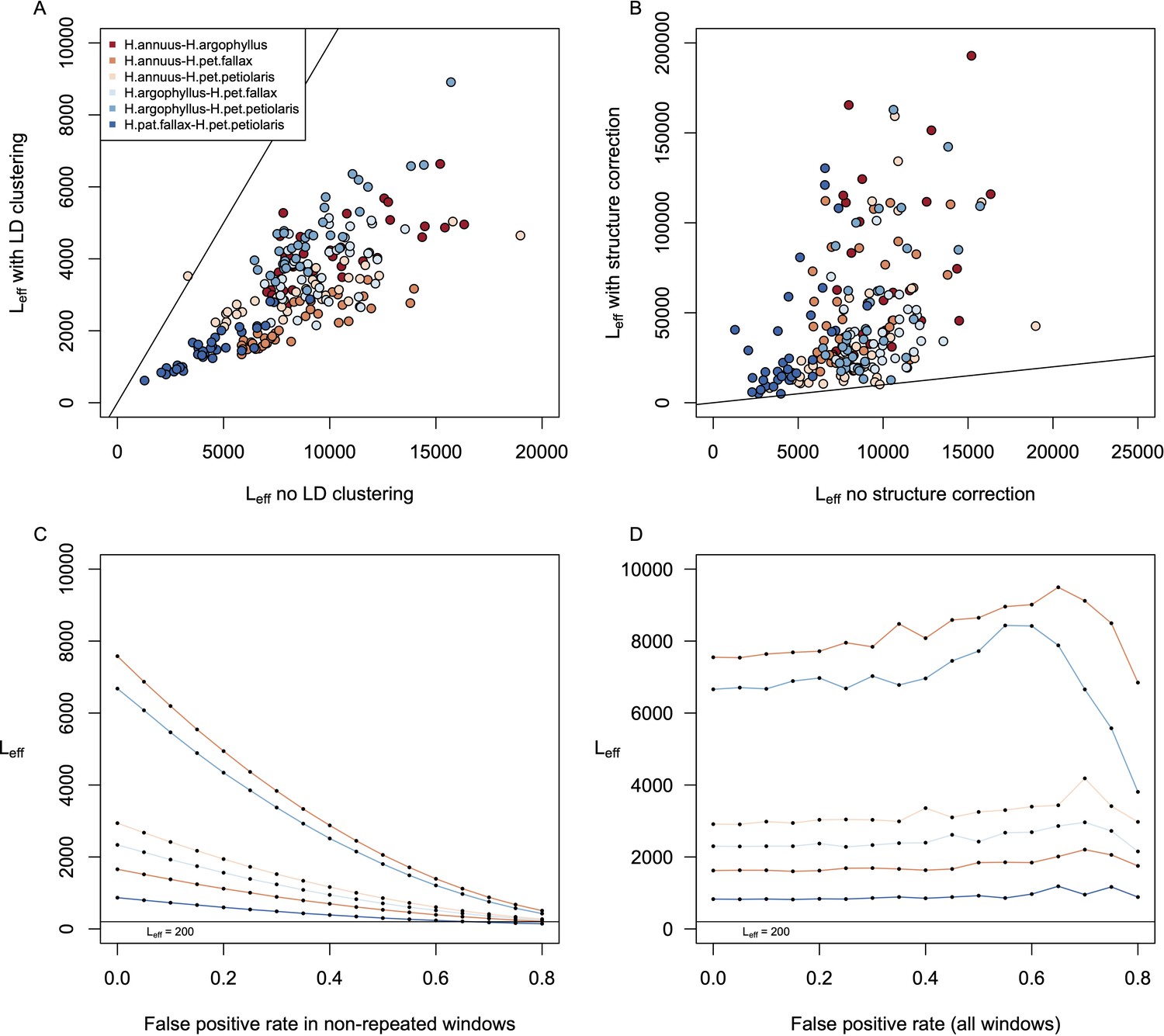
Estimates of effective number of loci in pairwise contrasts among species.
Panel (A) shows a comparison of estimates of the effective number of loci (Leff) when calculated with vs. without linkage disequilibrium (LD)-clustering for the environmental variables from the six pairwise contrasts among lineages. Panel (B) shows the effect of structure correction using BayPass on Leff. Panels (C) and (D) show the estimation of Leff for the variable with the lowest average value (Hargreaves reference evapotranspiration; Eref) under different false-positive rates for just the windows with non-repeated signatures (C) or for all windows (D).
Additional files
-
Supplementary file 1
Tables showing phenotypes and environmental variables for all sampled individuals and populations, as well as legends for details associated with each variable (reproduced from Todesco et al., 2020).
- https://cdn.elifesciences.org/articles/88604/elife-88604-supp1-v1.xlsx
-
MDAR checklist
- https://cdn.elifesciences.org/articles/88604/elife-88604-mdarchecklist1-v1.docx
Download links
A two-part list of links to download the article, or parts of the article, in various formats.
Downloads (link to download the article as PDF)
Open citations (links to open the citations from this article in various online reference manager services)
Cite this article (links to download the citations from this article in formats compatible with various reference manager tools)
Repeatability of adaptation in sunflowers reveals that genomic regions harbouring inversions also drive adaptation in species lacking an inversion
eLife 12:RP88604.
https://doi.org/10.7554/eLife.88604.3


