Disrupting abnormal neuronal oscillations with adaptive delayed feedback control
- Neuroengineering and Computational Neuroscience Lab, i3S - Instituto de Investigação e Inovação em Saúde, Universidade do Porto, Portugal
- Faculdade de Engenharia, Universidade do Porto, Portugal
- Department of Biomedical Engineering, University of Melbourne, Australia
Figures
Figure 1 with 1 supplement
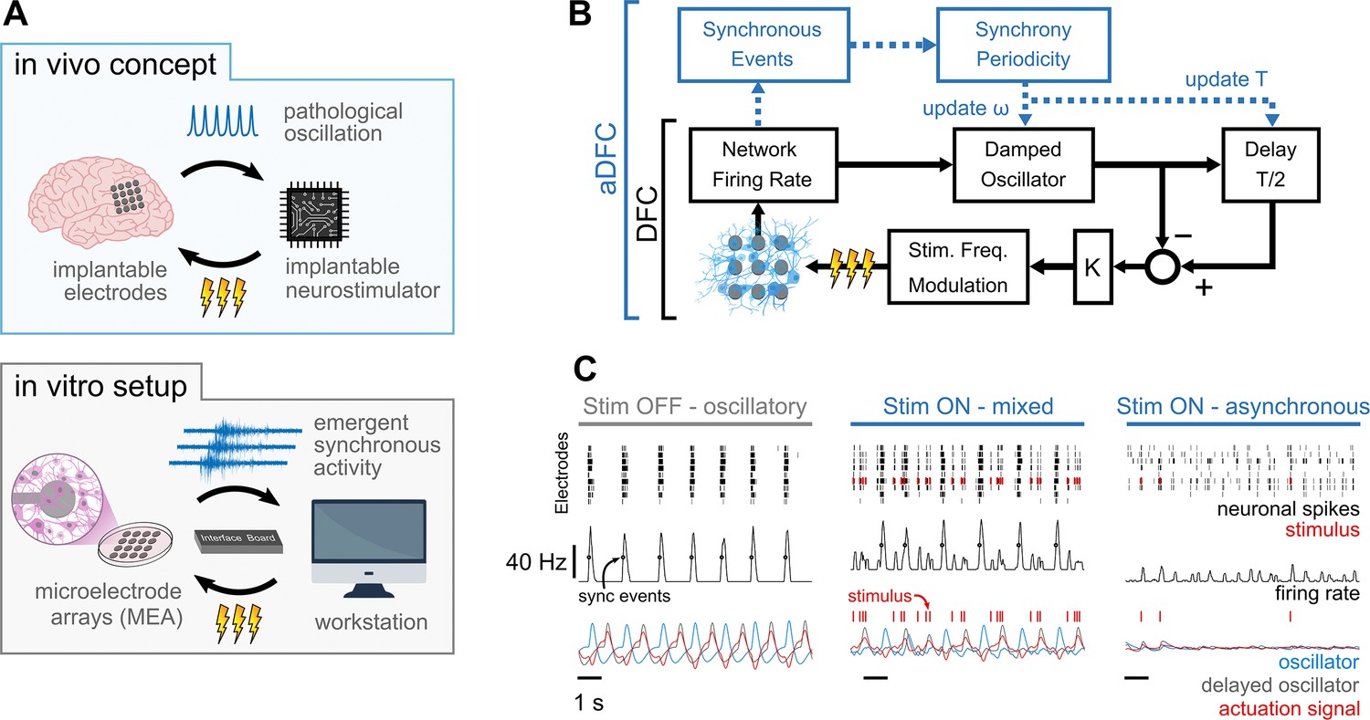
Controlling pathological oscillations with adaptive delayed feedback control (aDFC).
(A) In vivo concept of implantable closed-loop neurostimulation and the analogous in vitro setup developed. Here, we have dissociated hippocampal neurons as a brain, microelectrode arrays as implantable electrodes, emergent periodic network bursting as pathological synchronous oscillations, a workstation as an implantable chip, and an external stimulator as an implantable neurostimulator. (B) Scheme of the DFC algorithms. The instantaneous population firing rate is calculated and filtered by a damped oscillator. The actuation signal (stimulation frequency) is obtained by subtracting the ongoing oscillation from the past half-cycle delayed oscillation. The natural frequency of the oscillator, ω, and the duration of the half-cycle delay are updated online (adaptive component in blue) by detecting the synchronous events and their current periodicity, T. (C) Controller computations under different firing regimes – oscillatory (left), asynchronous (right), and mixed, i.e., oscillatory with induced sparse activity (middle). Spike detection is performed for the monitoring electrodes (top) and the spike train is convolved online with a square window to compute the instantaneous population firing rate (middle). Synchronous events (black circles) are detected using a threshold crossing method and used to update the oscillation periodicity. The actuation signal (red) is built by subtracting the oscillator and delayed oscillator signals (blue and grey, respectively) and translated to a stimulation frequency signal.
Figure 1—figure supplement 1
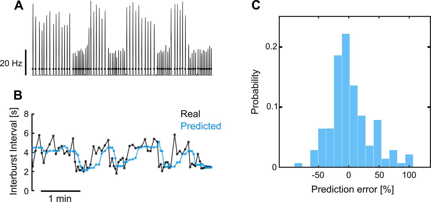
Representative example of adaptive delayed feedback control (aDFC) adaptability in a network with fast-changing dynamics.
(A) Instantaneous network firing rate during spontaneous activity. The black dots represent the real-time detection of network bursts performed by the adaptive controller. (B) Inter-burst interval predicted by the aDFC controller and the associated real inter-bursts. Every time the controller detects a new network burst (black dots in A) it estimates when the next burst would spontaneously occur by calculating the median of the previous five inter-burst intervals. This prediction is used to properly tune the controller’s half-cycle delay and the natural frequency of the oscillators used to create the actuation signal. In this example the stimulation is turned OFF, so the controller is simply tracking the neuronal activity without interfering with it. (C) Histogram of the prediction error for the representative example shown in A and B. The largest errors result from the prediction lag associated with the fast transitions between bursting regimes. The fact that the prediction error is typically small, even under these fast-changing network dynamics, means that the half-cycle delay and the oscillator’s natural frequency of aDFC are properly self-tuned in real time.
Figure 2
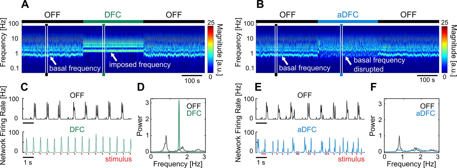
Representative example of the effect of delayed feedback control (DFC) and adaptive DFC (aDFC) stimulation protocols.
(A, B) Wavelet transform of the instantaneous firing rate of a network under DFC (A) and aDFC (B) protocols. (C, E) Example of the instantaneous firing rate of the network before stimulation (black) and during DFC (C, green) and aDFC (E, blue) stimulation. The signals shown in C and E correspond to the narrow time windows marked in A and B, respectively. (D, F) Power spectrum density of the instantaneous firing rate of the network before stimulation (black) and during DFC (D, green) and aDFC (F, blue) stimulation.
Figure 3 with 3 supplements
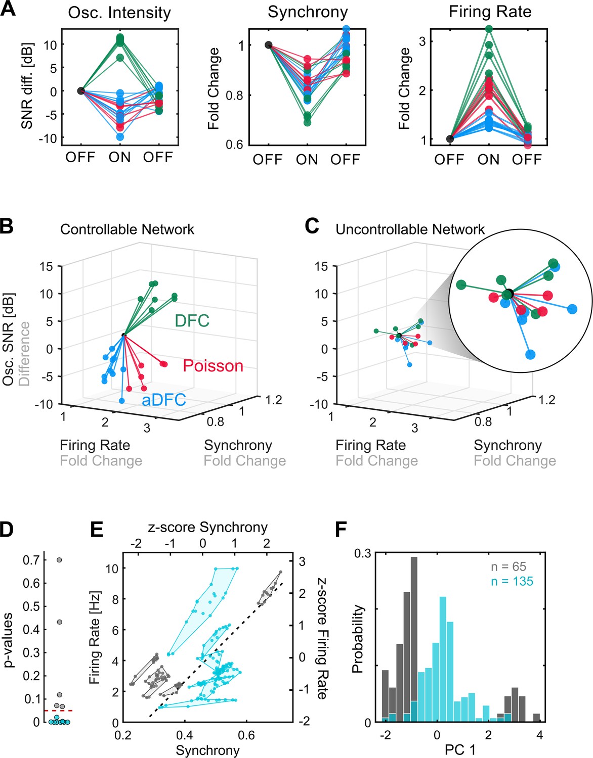
Comparison of controllable and uncontrollable networks.
(A) Results obtained from multiple repetitions of the three stimulation protocols for a single network. We calculated the synchrony, firing rate, and oscillation intensity for the three segments – pre-stimulation (OFF), stimulation (ON), post-stimulation (OFF) – of each experiment and normalised each metric to the value of the pre-stimulation period. For the oscillation intensity, this normalisation corresponds to the difference and not ratio, since the signal-to-noise ratio (SNR) is given in dB (logarithmic scale). Each triplet of points corresponds to one experiment performed with either adaptive delayed feedback control (aDFC) (blue), DFC (green), or Poisson (red) stimulation. (B) Three-dimensional (3D) feature space – firing rate vs. synchrony vs. oscillation intensity – for the network in A. Each line corresponds to the metrics evolution from the initial OFF to ON (from the first to the second point in A). This network is considered controllable since each protocol consistently drove the network to a distinct subspace, meaning that it had a unique and reproducible effect. (C) Representative example of the 3D feature space for an uncontrollable network where the effect of each stimulation protocol is indistinguishable from the others. (D) Networks were separated into controllable (blue) and uncontrollable (grey) by computing the multivariate ANOVA (MANOVA) of the ON metrics for the different stimulation protocols. Networks with p-values lower than 0.05 had separable effects in the 3D feature space of the metrics and were thus considered controllable (8/13). (E) Pre-stimulation firing rate and synchrony for all experiments performed with each network, divided into controllable and uncontrollable networks. Each dot corresponds to one experiment performed with either DFC, aDFC, or Poisson in a given network. The experiments performed with the same network are confined in a polygon. The black traced line corresponds to the first principal component (PC1) of the standardised (z-score, i.e. mean equals zero and standard deviation equals one) synchrony and firing rate defining a relevant descriptor of the neuronal dynamics. (F) Distribution of the baseline neuronal dynamics along PC1, defined in E, showing that the controllable networks have an intermediate level of spontaneous firing rate and synchrony.
Figure 3—figure supplement 1
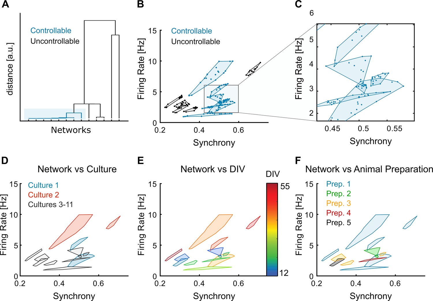
Controllable and uncontrollable networks across cultures, DIVs, and animal preparations.
(A) Dendrogram of the networks according to the controllability measure (multivariate ANOVA [MANOVA] p-values of the modulation results obtained with the different stimulation protocols). This representation shows that the controllable networks (p-values <0.05) are more similar to each other than to the uncontrollable ones. (B) Spontaneous firing rate and synchrony for the all the trials of the different networks, separated into controllable and uncontrollable networks. (C) Detail of B, evidencing how some cultures have very well-confined spontaneous dynamics. (D) Division of the networks according to the associated neuronal culture. When probed in different days, the same neuronal culture can be considered a different dynamical system because the spontaneous dynamics are clearly different. Therefore, we consider these to be different networks. For example, culture 1 (blue) and culture 2 (orange) led to two different networks each and, in the case of culture 2 one network is controllable whereas the other is not. Cultures 3–11 (grey) only have one network each and are represented with the same colour for clarity. (E) Evolution of the networks with the DIV. Also, the DIV by itself does not predict which networks are controllable and uncontrollable as these groups span multiple overlapping DIVs. (F) The networks used came from a total of five different animal preparations. The distinction of controllable and uncontrollable networks cannot be attributed to any particular preparation, as the same preparation can lead to both types of networks.
Figure 3—figure supplement 2
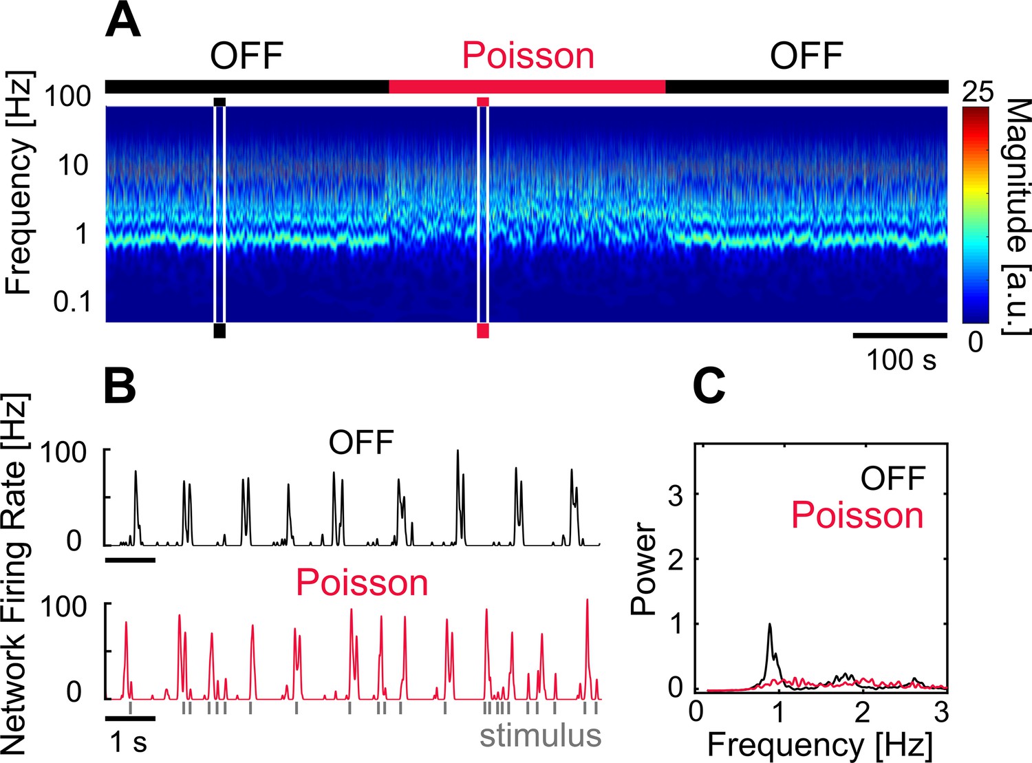
Representative example of the effect of Poisson stimulation in the frequency domain.
(A) Wavelet transform of the instantaneous network firing rate during the OFF and ON periods. (B) Example of the instantaneous firing rate of the network before stimulation (black) and during Poisson stimulation. The signals shown in B correspond to the narrow time windows marked in A. (C) Power spectrum density of the instantaneous firing rate of the network before stimulation (black) and during Poisson stimulation. Since the random Poisson stimulation is an open-loop control algorithm, i.e., it does not adapt to the ongoing network dynamics, the frequency of the Poisson process (which triggers the stimulation) had tuned beforehand. For that, we set the average stimulation frequency to match the average stimulation frequency used in the antecedent adaptive delayed feedback control (aDFC) experiment. It is important to note that, even if properly tuned, open-loop Poisson stimulation will not adjust as the network approaches the desired state or stop stimulating once it is reached. This is relevant for cases like the one displayed in Figure 7, where aDFC and Poisson stimulation led to very different network responses.
Figure 3—figure supplement 3
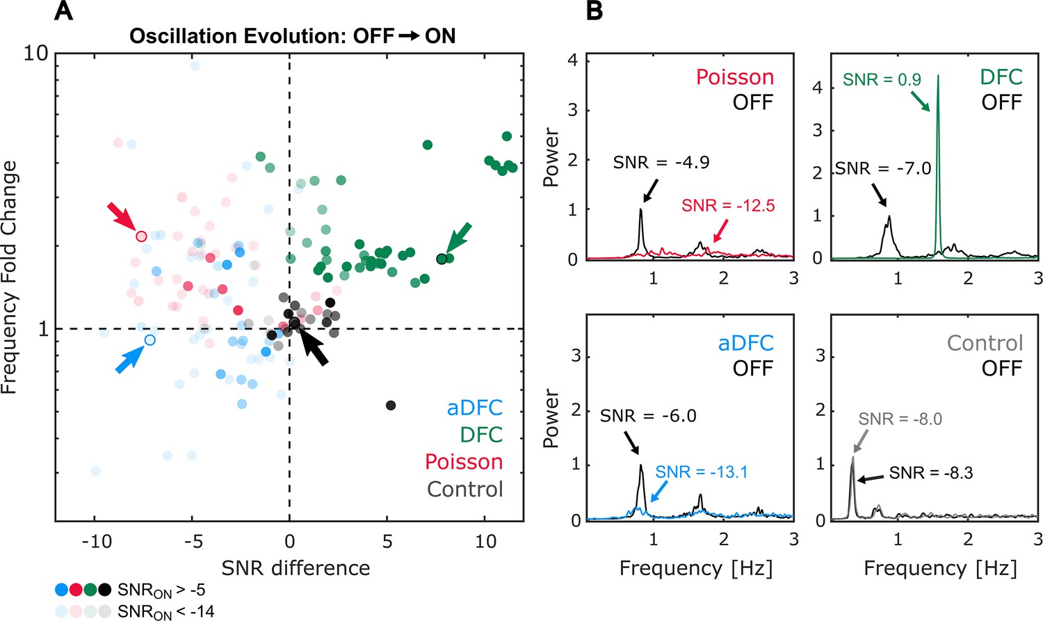
Delayed feedback control (DFC) leads to an increase in oscillation intensity and frequency.
(A) Change in oscillation frequency (fold change) as a function of the change in oscillation intensity (signal-to-noise ratio [SNR] difference) from the OFF to ON periods. In this representation, the left and right quadrants are respectively associated with a decrease and increase in oscillation intensity when stimulation is turned ON. The lower and upper quadrants are respectively associated with a reduction and increase in the oscillation frequency during stimulation. The oscillation frequency corresponds to the frequency at the peak of the power spectrum density (PSD). To account for the fact that oscillations with very low SNR may not have a meaningfull value of oscillation frequency, the opacity of the datapoints is proportional to the value of SNR during the ON period. Thus, the more transparent points have less meaningful values of oscillation frequency. Each datapoint corresponds to an individual experiment performed with a given controllable network and stimulation protocol (adaptive DFC [aDFC] in blue, DFC in green, Poisson in red, and control in grey). The experiments performed with DFC are mostly located on the upper right quadrant, meaning that it consistently leads faster and more consistent oscillations. aDFC and random stimulation lead to a decrease in oscillation intensity, and the oscillation frequency is typically neglectable (datapoints are mostly transparent). As expected, the control group, where no stimulation is applied, is located at the centre of the map, since the activity is similar during the ON and OFF periods. (B) Representative examples of the PSD, from where the oscillation intensity and frequency are calculated, during the OFF and ON periods for the three stimulation protocols and control, marked with arrows in panel A.
Figure 4 with 1 supplement
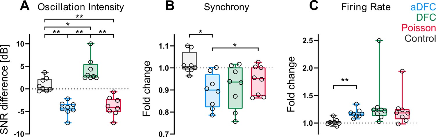
Effect of adaptive delayed feedback control (aDFC), DFC, and Poisson stimulation in controllable networks.
Fold change in oscillation intensity (A), synchrony (B), and firing rate (C) of the 5 min stimulation period compared to the 5 min pre-stimulation period with aDFC (blue), DFC (green), and Poisson (red) stimulation. The control group (grey) corresponds to baseline recordings where there is no stimulation and thus portrays the natural variability of each metric within two subsequent 5 min blocks. Each point represents the average effect of a stimulation protocol across all trials for a given network. We used the one-way ANOVA with repeated measures as statistical test (n=8; *p<0.05; **p<0.01; details of statistical tests in Supplementary file 1 [Table S1]).
Figure 4—figure supplement 1

Adaptive delayed feedback control (aDFC) allows the network to maintain some autonomous firing whereas DFC and Poisson tend to confine most network activity to stimulus responses.
(A) Stimuli (red) and respective response windows of 400 ms (blue) for representative examples of aDFC (top), DFC (middle), and Poisson (bottom) applied to the same network. (B) Detail of the spikes (black) evoked after stimulation (red) inside the response window (blue). (C) Fraction of evoked spikes during stimulation for all the trials performed with the three protocols for each controllable network (one plot per network). When the fraction of evoked spikes is close to 1, the network has almost no spontaneous activity and is simply replicating the actuation signal, which is not ideal. (D) Comparison of the mean fraction of evoked spikes for the controllable networks. Each triplet of point corresponds to one network. aDFC has a significantly lower percentage of evoked activity, meaning that it allows the network to maintain some intrinsic activity. We used the one-way ANOVA with repeated measures as statistical test (n=p<0.05; **p<0.01; details of statistical tests in Supplementary file 3 [Table S3]). (E) Average stimulation frequency used by each method for all trials performed with all networks. The overall stimulation frequency is within the same range for all methods. This shows that the results found in D are not explained by differences in the amount of stimulation but are rather due to the specific timing of the stimuli determined by each algorithm.
Figure 5 with 1 supplement
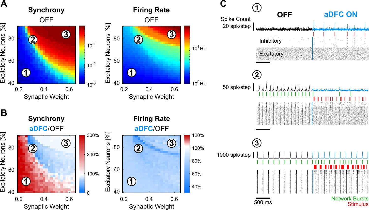
In silico networks also present a controllable subspace for intermediate baseline levels of firing rate and synchrony.
(A) Level of synchrony (left) and firing rate (right) for the period of spontaneous activity. Each pixel represents the average synchrony and firing rate of five different simulations under the same conditions of excitatory/inhibitory balance and synaptic weight. (B) Average change in synchrony (left) and firing rate (right) of adaptive delayed feedback control (aDFC) ON period compared to the OFF period. (C) Representative example of the simulations under three distinct network parameterisations (1, 2, and 3 in A and B). Each panel has the instant spike count at the top, the raster plot at the bottom, and the network bursts (green) and triggered stimuli (red) in the middle.
Figure 5—figure supplement 1
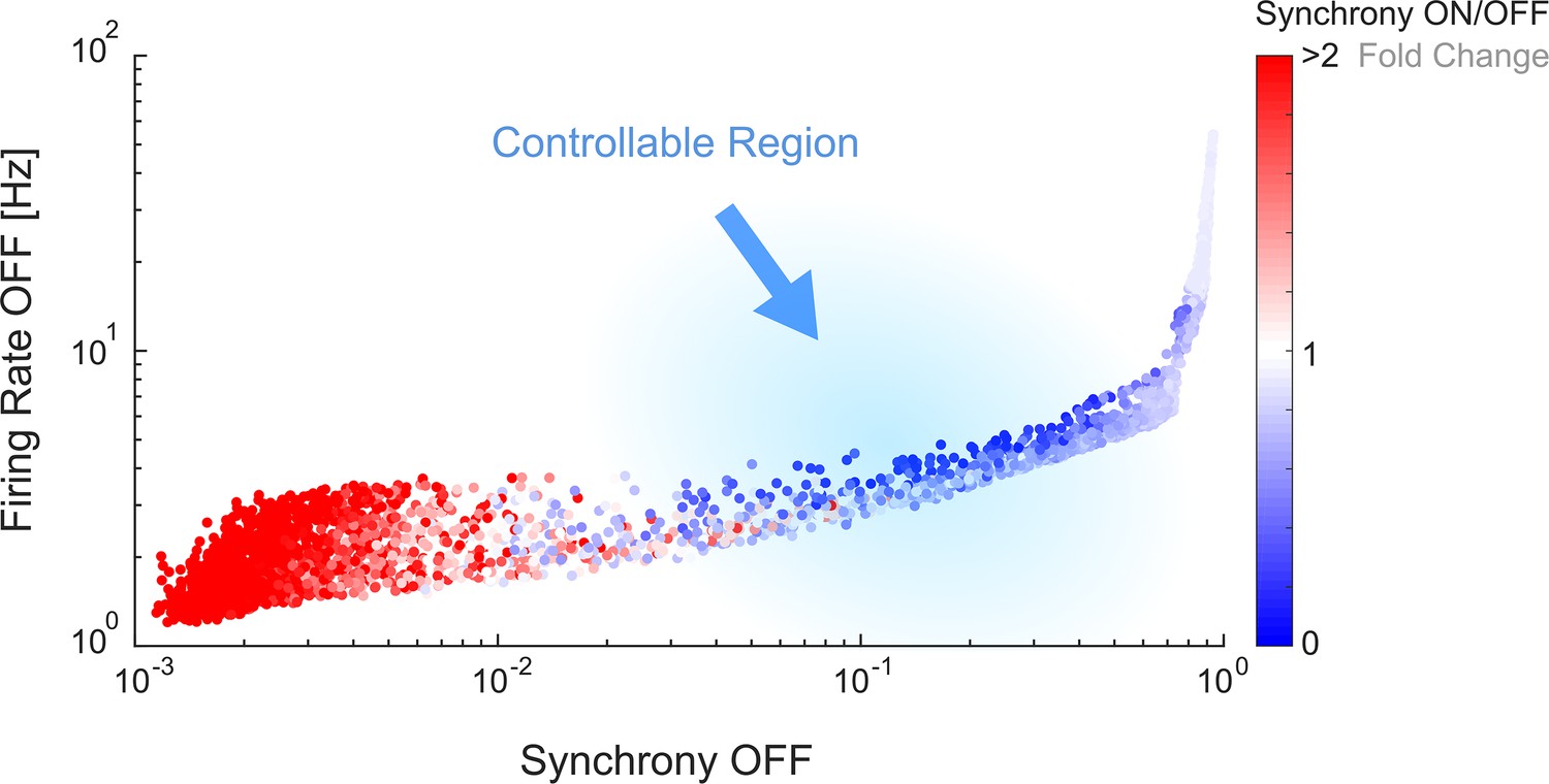
The controllable region of in silico networks is also associated with intermediate levels of spontaneous firing rate and synchrony.
The values of synchrony and firing rate during the initial OFF period were plotted for all the simulations performed, covering all the network parameterisations. The datapoints are coloured according to the change in synchrony level from OFF to ON, as a proxy for controllability. The in silico simulations cover a much larger metric space than the in vitro results, which are confined to the regions between a spontaneous synchrony of 10–1 and 100 and spontaneous firing rate of 100 and 101 (the in silico simulations with very low spontaneous synchrony generated firing dynamics that would not be elected for in vitro experiments).
Figure 6
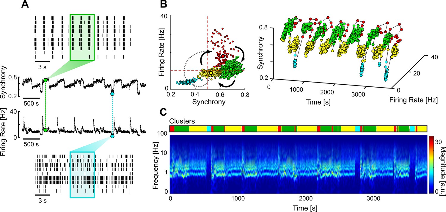
Multi-stable network with sporadic transitions to asynchronous state.
(A) Spontaneous synchrony and firing rate over time (middle). Representative raster plots of the synchronous (top) and asynchronous states (bottom). The coloured boxes represent the sliding window over which the firing rate and synchrony are calculated. (B) Synchrony vs. firing rate phase plot evidencing the cyclic behaviour of the network, with sporadic transitions to the asynchronous state (blue cluster). The clusters were identified using unsupervised Gaussian mixture models. (C) Changes in the frequency domain correlate with the automatically identified clusters (top bar).
Figure 7
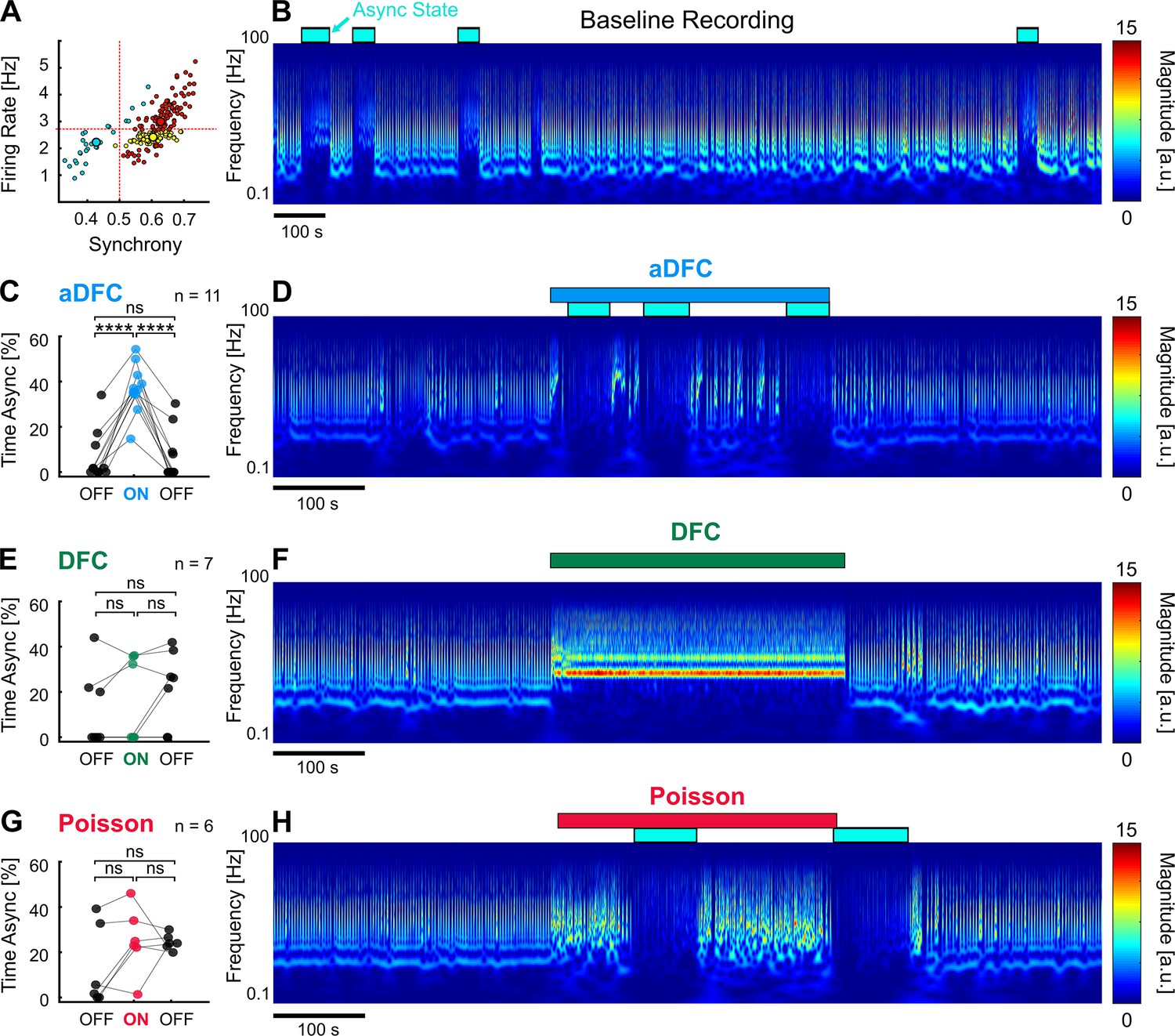
Adaptive delayed feedback control (aDFC) can promote transition to asynchronous state (AS).
(A) States of spontaneous activity for a given multi-stable network. Blue cluster represents the sporadically reached AS. (B) Frequency domain of the recording considered in A. Blue rectangles represent the regions associated with the automatically identified AS. (C, E, G) Percentage of time in AS during the OFF-ON-OFF protocols for aDFC (C), DFC (E), and Poisson (G) stimulation. Each triplet of points represents an experiment performed with the corresponding stimulation protocol. We compared the time spent in AS during the ON and OFF periods using one-way ANOVA with repeated measures (****p<0.0001; details of statistical tests in Supplementary file 2 [Table S2]). (D, F, H) Representative example of an experiment performed with aDFC (D), DFC (F), and Poisson (H) stimulation portrayed in the frequency domain. The stimulation period is represented with the associated coloured bar on the top. The identified AS are represented by the blue rectangles, as in B.
Additional files
-
Supplementary file 1
Details of the statistical tests used in Figure 4 to compare the modulation results of the different stimulation protocols in controllable networks.
We used repeated measures one-way ANOVA with multiple comparisons.
- https://cdn.elifesciences.org/articles/89151/elife-89151-supp1-v2.docx
-
Supplementary file 2
Details of the statistical tests used in Figure 7 to compare percentage of time spent in asynchronous state for each stimulation protocol in a multi-stable network.
We used repeated measures one-way ANOVA with multiple comparisons.
- https://cdn.elifesciences.org/articles/89151/elife-89151-supp2-v2.docx
-
Supplementary file 3
Details of the statistical tests used in Figure 3—figure supplement 2 to compare fraction of spontaneous spikes during stimulation for the three stimulation protocols.
We used repeated measures one-way ANOVA with multiple comparisons.
- https://cdn.elifesciences.org/articles/89151/elife-89151-supp3-v2.docx
-
MDAR checklist
- https://cdn.elifesciences.org/articles/89151/elife-89151-mdarchecklist1-v2.pdf
Download links
A two-part list of links to download the article, or parts of the article, in various formats.
Downloads (link to download the article as PDF)
Open citations (links to open the citations from this article in various online reference manager services)
Cite this article (links to download the citations from this article in formats compatible with various reference manager tools)
Disrupting abnormal neuronal oscillations with adaptive delayed feedback control
eLife 13:e89151.
https://doi.org/10.7554/eLife.89151


