Lotka-Volterra pairwise modeling fails to capture diverse pairwise microbial interactions

Version of Record

Accepted for publication after peer review and revision.

Download
Cite
Share
CommentOpen annotations (there are currently 0 annotations on this page).

Version of Record published: June 13, 2017 (This version)
Accepted Manuscript updated: April 3, 2017 (Go to version)
Accepted Manuscript published: March 28, 2017 (Go to version)
Accepted: March 18, 2017
Received: January 11, 2017

1. Of interest
Imputation of 3D genome structure by genetic–epigenetic interaction modeling in mice

Lauren Kuffler, Daniel A Skelly ... Gregory W Carter

Research Article Apr 26, 2024
Further reading

Abstract
eLife digest
Introduction
Results
Discussions
Materials and methods
References
Article and author information
Metrics

Abstract

Pairwise models are commonly used to describe many-species communities. In these models, an individual receives additive fitness effects from pairwise interactions with each species in the community ('additivity assumption'). All pairwise interactions are typically represented by a single equation where parameters reflect signs and strengths of fitness effects ('universality assumption'). Here, we show that a single equation fails to qualitatively capture diverse pairwise microbial interactions. We build mechanistic reference models for two microbial species engaging in commonly-found chemical-mediated interactions, and attempt to derive pairwise models. Different equations are appropriate depending on whether a mediator is consumable or reusable, whether an interaction is mediated by one or more mediators, and sometimes even on quantitative details of the community (e.g. relative fitness of the two species, initial conditions). Our results, combined with potential violation of the additivity assumption in many-species communities, suggest that pairwise modeling will often fail to predict microbial dynamics.

https://doi.org/10.7554/eLife.25051.001

eLife digest

From the soil to our body, microbes, such as bacteria, are everywhere and affect us in many ways. Many microbes perform important roles in natural environments and for our health, but some of them can cause harm and lead to diseases. Often, microbes affect and interact with each other within large groups or communities. Because of their widespread ramifications, it is important to understand how microbial communities work.

In addition to experiments, mathematical modeling offers one way to gain insight into the dynamics of microbial communities. A model commonly used to describe the interactions between organisms is the so-called ‘pairwise model’. Pairwise models can be useful to predict the dynamics of a community in which two species physically interact, such as a predator-prey community. However, it was unknown if this model was suitable to adequately predict the dynamics of microbial species in communities. Microbes often interact via chemicals that diffuse in the environment. For example, one microbe might provide food for another microbe or release toxins to kill it. However, a pairwise model does not consider food or toxins, but only how one microbe stimulates or inhibits the growth of another.

Momeni et al. simulated different scenarios commonly found in microbial communities to test whether a pairwise model could capture how, for example, chemicals released by one bacterial species would either help others to grow or stop them from growing. The results showed that for many scenarios, pairwise models cannot qualitatively represent the dynamics of a microbial community.

A next step will be to work on the limitations of current experimental technologies and mathematical models to improve the understanding of microbial communities. This knowledge could be used to develop new strategies for ecosystem engineering, such as for example making soils more fertile to improve crop yields, or tackling antibiotic resistance of bacteria.

https://doi.org/10.7554/eLife.25051.002

Introduction

Multispecies microbial communities are ubiquitous. Microbial communities are important for industrial applications such as cheese and wine fermentation (van Hijum et al., 2013) and municipal waste treatment (Seghezzo et al., 1998). Microbial communities are also important for human health: they can modulate immune responses and food digestion (Round and Mazmanian, 2009; Kau et al., 2011) during health and disease. Properties of the entire community (‘community properties’, e.g. species dynamics, ability to survive internal or external perturbations, and biochemical activities of the entire community) are influenced by interactions wherein individuals alter the physiology of other individuals (Widder et al., 2016). To understand and predict community properties, choosing the appropriate mathematical model to describe species interactions is critical.

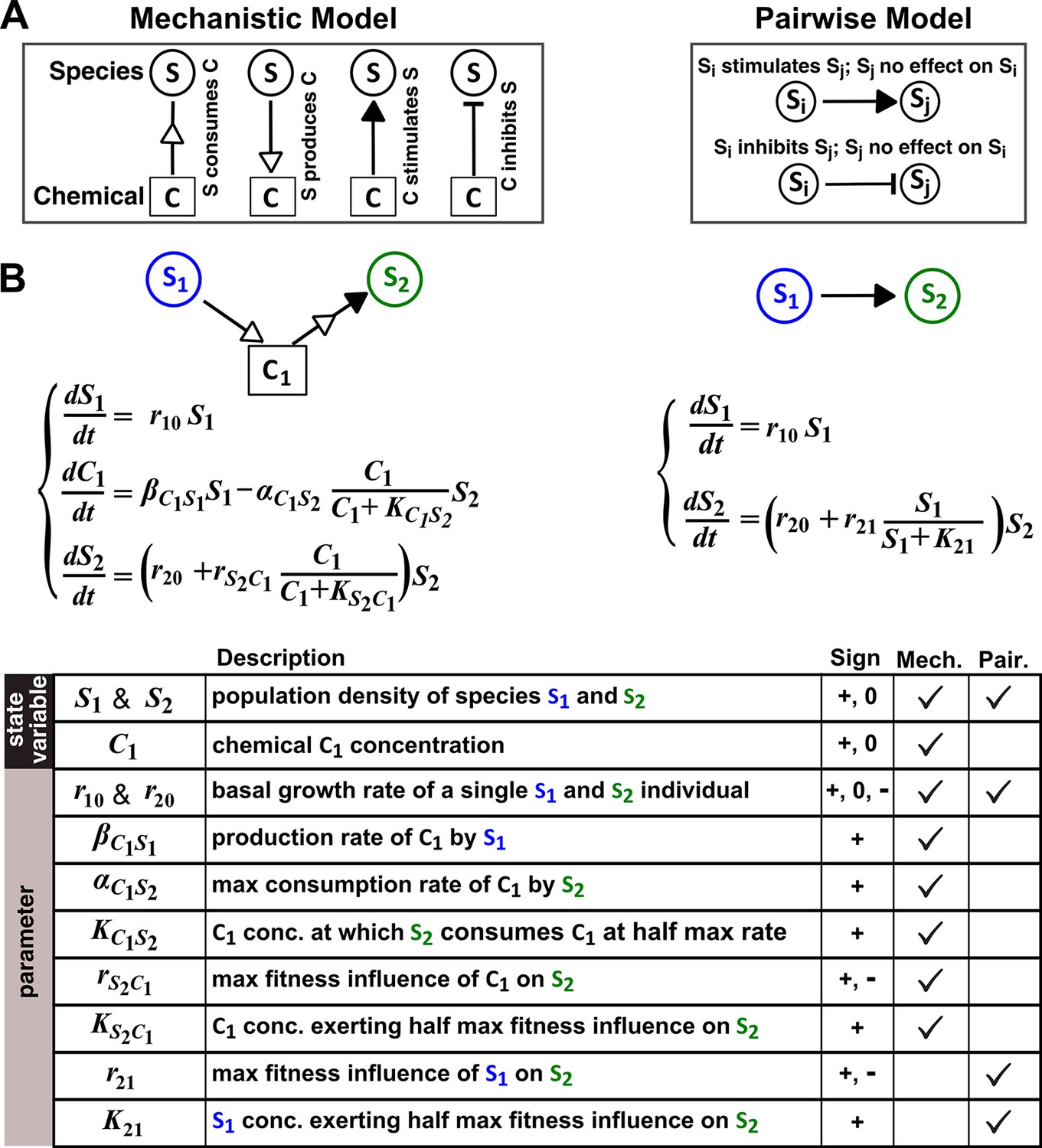
A mathematical model ideally focuses only on details that are essential to community properties of interest. However, it is often unclear a priori what the minimal essential details are. We define ‘mechanistic models’ as models that explicitly consider interaction mediators as state variables. For example, if species S₁ releases a compound C₁ which stimulates species S₂ growth upon consumption by S₂, then a mechanistic model tracks concentrations of S₁, C₁, and S₂ (Figure 1A and B, left panels). Note that mechanistic models used here still omit molecular details such as how chemical mediators are received and processed by recipients and how mediators subsequently act on recipients. In contrast, Lotka-Volterra (‘L-V’) pairwise models only consider the fitness effects of interactions. Specifically, L-V models assume that the fitness of an individual is the sum of its basal fitness (the net growth rate of an individual in isolation) and fitness influences from pairwise interactions with individuals of the same species and of every other species in the community (‘additivity’ assumption). Furthermore, regardless of interaction mechanisms or quantitative details of a community, all fitness influences are typically expressed using a single equation form wherein parameters can vary to reflect the signs and magnitudes of fitness influences (‘universality’ assumption). Thus in the example above, a pairwise model only describes how S₁ increases the fitness of S₂ (Figure 1A and B, right panels).

Figure 1 with 2 supplements see all

Download asset Open asset

The abstraction of interaction mechanisms in a pairwise model compared to a mechanistic model.

(A) The mechanistic model (left) considers a bipartite network of species and chemical interaction mediators. A species can produce or consume chemicals (open arrowheads pointing towards and away from the chemical, respectively). A chemical mediator can positively or negatively influence the fitness of its target species (filled arrowhead and bar, respectively). The corresponding L-V pairwise model (right) includes only the fitness effects of species interactions, which can be positive (filled arrowhead), negative (bar), or zero (line terminus). (B) In the example here, species S₁ releases chemical C₁, and C₁ is consumed by species S₂ and promotes S₂’s fitness. In the mechanistic model, the three equations respectively state that (1) S₁ grows exponentially at a rate $r_{10}$ , (2) C₁ is released by S₁ at a rate $β_{C_{1} S_{1}}$ and consumed by S₂ with saturable kinetics (maximal consumption rate $α_{C_{1} S_{2}}$ and half-saturation constant $K_{C_{1} S_{2}}$ ), and (3) S₂’s growth (basal fitness $r_{20}$ ) is influenced by C₁ in a saturable fashion. In the pairwise model here, the first equation is identical to that of the mechanistic model. The second equation is similar to the last equation of the mechanistic model except that $r_{21}$ and $K_{21}$ together reflect how the density of S₁ ( $S_{1}$ ) affects the fitness of S₂ in a saturable fashion. For all parameters with double subscripts, the first subscript denotes the focal species or chemical, and the second subscript denotes the influencer. Note that unlike in mechanistic models, we have omitted ‘ $S$ ’ from subscripts in pairwise models (e.g. $r_{21}$ instead of $r_{S_{2} S_{1}}$ ) for simplicity. In this example, both $r_{21}$ and $r_{S_{2} S_{1}}$ are positive.

https://doi.org/10.7554/eLife.25051.003

L-V pairwise models are popular. L-V pairwise modeling has successfully explained the oscillatory dynamics of hare and its predator lynx (Figure 1—figure supplement 1) (Volterra, 1926; Wangersky, 1978; BiologyEOC, 2016). Pairwise models have also been instrumental in delineating conditions for multiple carnivores to coexist when competing for herbivores (MacArthur, 1970; Chesson, 1990). In both cases, mechanistic models and pairwise models happen to be mathematically equivalent for the following reasons. In the hare-lynx example, both species are also interaction mediators, and therefore pairwise and mechanistic models are identical. In the second example, if herbivores (mediators of competitive interactions between carnivores) rapidly reach steady state, herbivores can be mathematically eliminated from the mechanistic model to yield a pairwise model of competing carnivores (MacArthur, 1970; Chesson, 1990). Pairwise models are often used to predict how perturbations to steady-state species composition exacerbate or decline over time (May, 1972; Thébault and Fontaine, 2010; Mougi and Kondoh, 2012; Allesina and Tang, 2012; Suweis et al., 2013; Coyte et al., 2015). Although most work are motivated by contact-dependent prey-predation (e.g. hare-lynx) or mutualisms (e.g. plant-pollinator) where L-V models could be identical to mechanistic models, these work do not explicitly exclude chemical-mediated interactions where species are distinct from interaction mediators.

The temptation of using pairwise models is indeed high, including in microbial communities where many interactions are mediated by chemicals (Mounier et al., 2008; Faust and Raes, 2012; Stein et al., 2013; Marino et al., 2014; Coyte et al., 2015). Even though pairwise models do not capture the dynamics of chemical mediators, predicting species dynamics is still highly desirable in, for example, forecasting species diversity and compositional stability. For chemical-mediated interactions, L-V pairwise models are far easier to construct than mechanistic models for the following reasons. Mechanistic models would require knowledge of chemical mediators, which are often challenging to identify. Since chemical mediators are explicitly modeled, mechanistic models require more equations and parameters than their cognate pairwise models (Figure 1, Table). Pairwise model parameters are relatively easy to estimate using community dynamics or dynamics of monocultures and pairwise cocultures (Mounier et al., 2008; Stein et al., 2013; Guo and Boedicker, 2016). Consequently, pairwise modeling has been liberally applied to microbial communities.

L-V pairwise models have been criticized when applied to communities of more than two species (referred to as ‘multispecies communities’) (Levine, 1976; Tilman, 1987; Wootton, 1993, 2002; Werner and Peacor, 2003; Stanton, 2003; Schmitz et al., 2004). This is because a third species can influence interactions between a species pair (‘indirect interactions’), which sometimes violates the additivity assumption of pairwise models. For example, a carnivore can indirectly increase the density of a plant by decreasing the density of an herbivore (‘interaction chain’; ‘density-mediated indirect interactions’). A carnivore can also decrease how often an herbivore forages plants (‘interaction modification’, ‘trait-mediated indirect interactions’, or ‘higher order interactions’) (Vandermeer, 1969; Wootton, 1994; Billick and Case, 1994; Wootton, 2002). In interaction modification, foraging per herbivore decreases, whereas in interaction chain, the density of herbivores decreases. Interaction modification (but not interaction chain) violates the additivity assumption (Methods-Interaction modification but not interaction chain violates the additivity assumption) (Tilman, 1987; Wootton, 1994; Schmitz et al., 2004) and can cause the pairwise model to generate qualitatively wrong predictions. Indeed, pairwise models largely failed to predict biomass and species coexistence in three-species and seven-species plant communities (Dormann and Roxburgh, 2005), although reported failures of pairwise models could be due to limitations in data collection and analysis (Case and Bender, 1981; Billick and Case, 1994).

Here, we examine the universality assumption of pairwise models when applied to microbial communities (or any community that employs diverse chemical-mediated interactions). Microbes often influence other microbes in a myriad of fashions, via consumable metabolites, reusable signaling molecules, or a combination of chemicals (Figure 2). Can a single equation form, traditionally employed in pairwise models, qualitatively describe diverse interactions between two microbial species? The answer is unclear. On the one hand, pairwise models have been applied successfully to diverse microbial communities. For example, an L-V pairwise model and a mechanistic model both correctly predicted ratio stabilization and spatial intermixing between two strongly-cooperating populations exchanging diffusible essential metabolites (Momeni et al., 2013). In other examples, pairwise models largely captured competition outcomes and metabolic activities of three-species and four-species artificial microbial communities (Vandermeer, 1969; Guo and Boedicker, 2016; Friedman et al., 2017). On the other hand, pairwise models often failed to predict species coexistence in seven-species microbial communities (Friedman et al., 2017), although this could be due to interaction modification discussed above.

Figure 2

Download asset Open asset

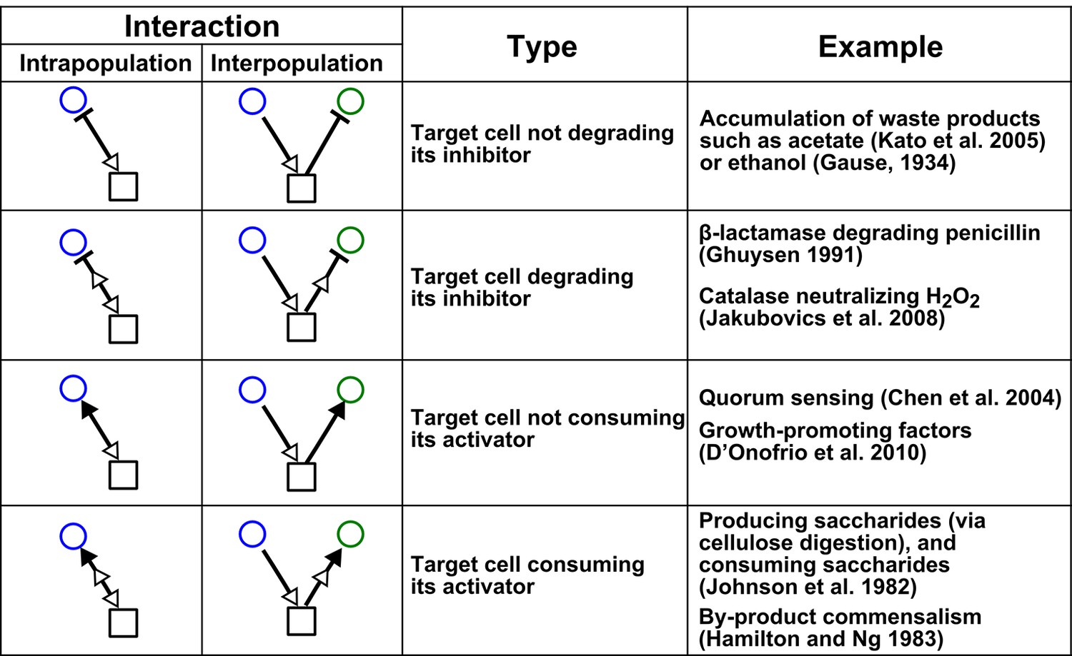
Chemical-mediated interactions commonly found in microbial communities.

Interactions can be intra- or inter-population. Examples are meant to be illustrative instead of comprehensive.

https://doi.org/10.7554/eLife.25051.006

Instead of investigating natural communities where interaction mechanisms can be difficult to identify, we use in silico communities. In these communities, two species interact via mechanisms commonly encountered in microbial communities, including growth-promoting and growth-inhibiting interactions mediated by reusable and consumable compounds (Figure 2) (Stams, 1994; Czárán et al., 2002; Duan et al., 2009). We construct mechanistic models for these two-species communities and attempt to derive from them pairwise models. A mechanistic reference model offers several advantages: community dynamics is deterministically known; deriving a pairwise model is not limited by inaccuracy of experimental methods; and the flexibility in creating different reference models allows us to explore a variety of interaction mechanisms. We demonstrate that a single pairwise equation form often fails for commonly-encountered diverse pairwise microbial interactions. We conclude by discussing when pairwise models might or might not be useful, in light of our findings.

Results

Throughout this work, we consider communities grown in a well-mixed environment where all individuals interact with each other with an equal chance. A well-mixed environment can be found in industrial fermenters. Moreover, at a sufficiently small spatial scale, a spatially-structured environment can be approximated as a well-mixed environment, as chemicals are uniformly-distributed locally. Motile organisms also reduce the degree of spatial structure. A well-mixed environment allows us to use ordinary differential equations (ODEs), which are more tractable than partial differential equations demanded by a spatially-structured environment. This in turn allows us to sometimes analytically demonstrate failures of pairwise models.

Mechanistic model versus pairwise model

A mechanistic model describes how species release or consume chemicals and how chemicals stimulate or inhibit species growth (Figure 1A left). In contrast, in pairwise models, interation mediators are not explicitly considered (Figure 1A right). Instead, the growth rate of an individual of species S_i is the sum of its basal fitness ( $r_{i 0}$ , net growth rate of the individual in the absence of any intra-species or inter-species interactions) and fitness effects from intra-species and inter-species interactions. The fitness effect from species S_j to species S_i is represented by $f_{i j} (S_{j})$ , where $S_{j}$ is the density of species S_j. $f_{i j} (S_{j})$ is a linear or nonlinear function of only $S_{j}$ and not of another species. When $j = i$ , $f_{i i} (S_{i})$ represents density-dependent fitness effect within S_i (e.g. density-dependent growth inhibition or stimulation).

In a multi-species pairwise model, a single form of $f_{i j}$ is used for all pairwise species interactions. For example, the most popular L-V model is linear L-V:

\frac{d S_{i}}{d t} = [r_{i 0} + \sum_{j} r_{i j} S_{j}] S_{i}

Here, $r_{i 0}$ is the basal fitness of an individual of S_i, and can be positive, negative, or zero; $r_{i j}$ is the fitness effect per S_j individual on S_i. Positive, negative, or zero $r_{i j}$ represents growth stimulation, inhibition, or no effect, respectively. An example of linear L-V is the logistic L-V pairwise model traditionally used for competitive communities:

\frac{d S_{i}}{d t} = r_{i 0} [1 - \sum_{j} \frac{S_{j}}{Λ_{i j}}] S_{i}

Here, nonnegative $r_{i 0}$ is the basal fitness of S_i; positive $Λ_{i j}$ is the carrying capacity imposed by limiting shared resource (e.g. space or carbon source) such that a single S_i individual will have a zero net growth rate when competing with a total of $Λ_{i j}$ individuals of S_j.

Alternative forms of fitness effect $f_{i j}$ (Wangersky, 1978) include L-V with delayed influence, where the fitness influence of one species on another may lag in time (Gopalsamy, 1992), or saturable L-V (Thébault and Fontaine, 2010) where

\frac{d S_{i}}{d t} = [r_{i 0} + \sum_{j} r_{i j} \frac{S_{j}}{K_{i j} + S_{j}}] S_{i}

Here, $r_{i 0}$ is the basal fitness of an individual of S_i, $r_{i j}$ is the maximal fitness effect species S_j can exert on S_i, and $K_{i j}$ (>0) is the $S_{j}$ at which half maximal fitness effect on S_i is achieved. $r_{i 0}$ and $r_{i j}$ can be positive, negative, or zero. Note that at a low concentration of influencer, the saturable form can be converted to a linear form.

Our goal is to test whether a single equation form of pairwise model can qualitatively predict dynamics of species pairs engaging in various types of interactions commonly found in microbial communities (e.g. Figure 2). To do so, we use a combination of analytical and numerical approaches (Figure 1—figure supplement 2). Analytically deriving a pairwise model from a mechanistic model not only reveals assumptions required to generate the pairwise model, but also alleviates any concern that we may have failed to identify the optimal pairwise model parameters. When interactions become more complex (e.g. involving multiple mediators), we take the numerical approach, which is typically used to infer pairwise models from experimental results (Pascual and Kareiva, 1996). In the numerical approach, we mimic experimentalists by first deciding on a pairwise model to be used, and then employing a nonlinear least squares routine to numerically identify model parameters that minimize the average difference $\bar{D}$ between pairwise and mechanistic model dynamics within a training time window $T$ (Figure 1—figure supplement 2; Methods-Summary of simulation files). To evaluate how well a pairwise model predicts long-term mechanistic model dynamics, we ‘buy time’ by introducing 'dilutions' in numerical simulations of both models and quantify their difference $\bar{D}$ .

Reusable versus consumable mediators require different pairwise models

In this section, we analytically derive pairwise models from mechanistic models of two-species communities where one species affects the other species through a single mediator. The mediator is either reusable such as signaling molecules in quorum sensing (Duan et al., 2009; Jakubovics, 2010) or consumable such as metabolites (Stams, 1994; Freilich et al., 2011) (Figure 2). We show that a single pairwise model may not encompass these different interaction mechanisms and that for consumable mediator, the choice of pairwise model also depends on details such as the relative fitness and initial densities of the two species.

Consider a commensal community where species S₁ stimulates the growth of species S₂ by producing a reusable (Figure 3A) or a consumable (Figure 3B) chemical C₁. We consider community dynamics where species are not limited by any abiotic resources, such as within a dilution cycle of a turbidostat experiment where all other metabolites are in excess.

Figure 3 with 5 supplements see all

Download asset Open asset

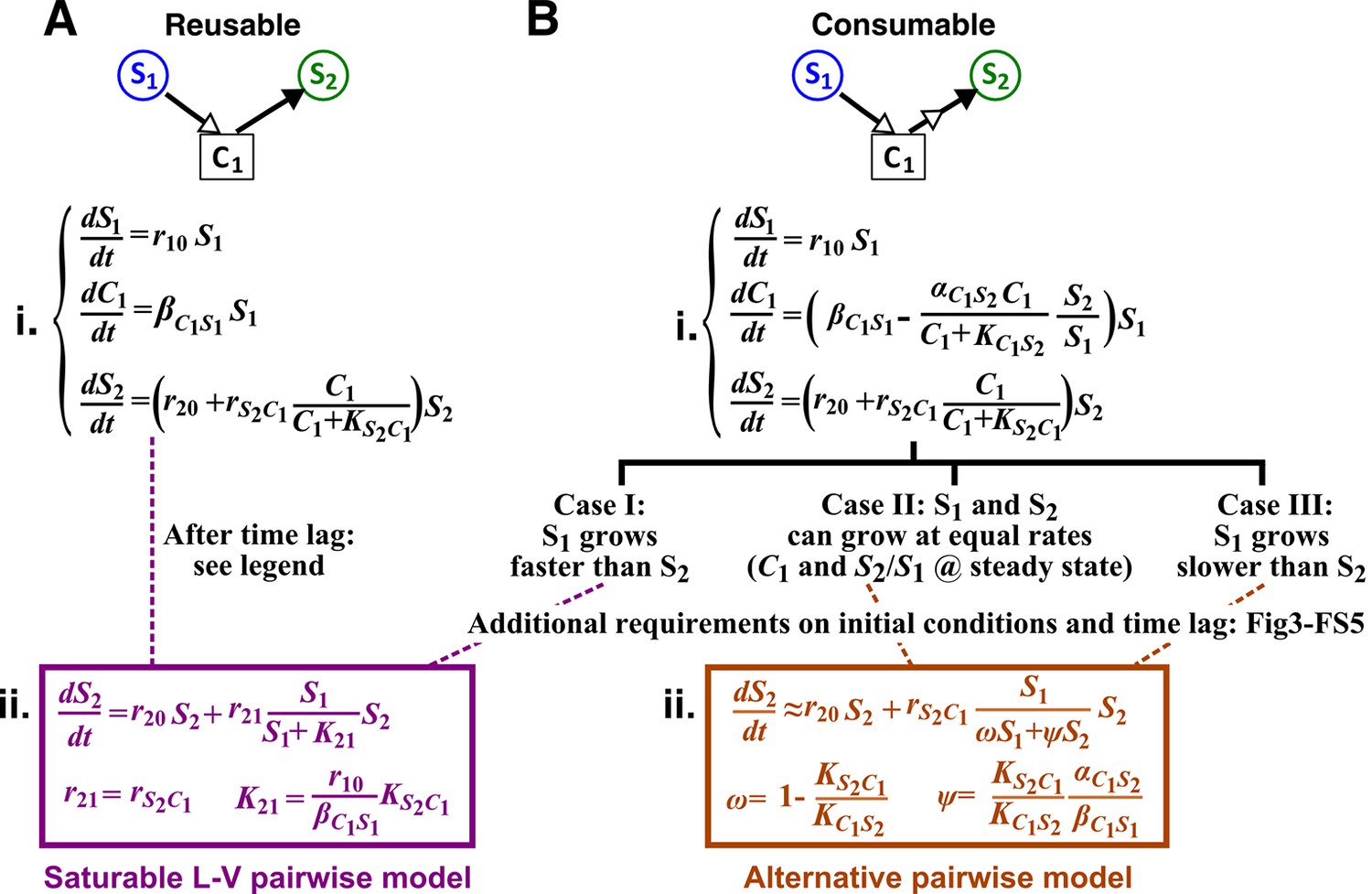
Interactions mediated via a single mediator are best represented by different forms of pairwise models, depending on whether the mediator is consumable or reusable and on the relative fitness and initial densities of the two species.

S₁ stimulates the growth of S₂ via a reusable (A) or a consumable (B) chemical C₁. In mechanistic models of the two cases (i), equations for $S_{1}$ and $S_{2}$ are identical but equations for $C_{1}$ are different. In (A), $C_{1}$ can be solved to yield $C_{1} = (β_{C_{1} S_{1}} / r_{10}) S_{10} \exp (r_{10} t) - (β_{C_{1} S_{1}} / r_{10}) S_{10} = (β_{C_{1} S_{1}} / r_{10}) S_{1} - (β_{C_{1} S_{1}} / r_{10}) S_{10}$ , assuming zero initial $C_{1}$ . Here, $S_{10}$ is $S_{1}$ at time zero. We have approximated $C_{1}$ by omitting the second term (valid after the initial transient response has passed so that $C_{1}$ has become proportional to $S_{1}$ ). This approximation allows an exact match between the mechanistic model and the saturable L-V pairwise model (ii). In (B), depending on the relative growth rates of the two species, and if additional requirements are satisfied (Methods; Figure 3—figure supplement 2; Figure 3—figure supplement 3; Figure 3—figure supplement 4; Figure 3—figure supplement 5), either saturable L-V or alternative pairwise model should be used.

https://doi.org/10.7554/eLife.25051.007

Figure 3—source data 1 List of parameters for simulations in Figure 3—figure supplement 1.: https://doi.org/10.7554/eLife.25051.008
Download elife-25051-fig3-data1-v3.docx
Figure 3—source data 2 List of parameters for simulations in Figure 3—figure supplement 2 on interactions through a consumable mediator.: https://doi.org/10.7554/eLife.25051.009
Download elife-25051-fig3-data2-v3.docx
Figure 3—source data 3 List of parameters for simulations in Figure 3—figure supplement 3 on conditions required for convergence of the alternative pairwise model.: https://doi.org/10.7554/eLife.25051.010
Download elife-25051-fig3-data3-v3.docx
Figure 3—source data 4 List of parameters for simulations in Figure 3—figure supplement 4 on how dilution might affect the convergence of a pairwise model.: https://doi.org/10.7554/eLife.25051.011
Download elife-25051-fig3-data4-v3.docx

When C₁ is reusable, the mechanistic model (Figure 3A,i) can be transformed into a saturable L-V pairwise model (compare Figure 3A,ii with Equation 3), especially after the concentration of the mediator (which is initially zero) has acclimated to be proportional to the producer population size (Figure 3A legend; Figure 3—figure supplement 1). This saturable L-V pairwise model is valid regardless of whether the producer coexists with the consumer, outcompetes the consumer, or is outcompeted by the consumer.

If C₁ is consumable, different scenarios are possible (Figure 3B; Methods).

Case I: When supplier S₁ always grows faster than consumer S₂ (the basal fitness of S₁ is higher than the maximal fitness of S₂), $C_{1}$ will eventually accumulate proportionally to $S_{1}$ (Figure 4A left; Methods-Deriving a pairwise model for interactions mediated by a single consumable mediator Case I). In this case, C₁ may be approximated as a reusable mediator and can be predicted by the saturable L-V pairwise model (Figure 4A right, compare dotted and solid lines).

Figure 4

Download asset Open asset

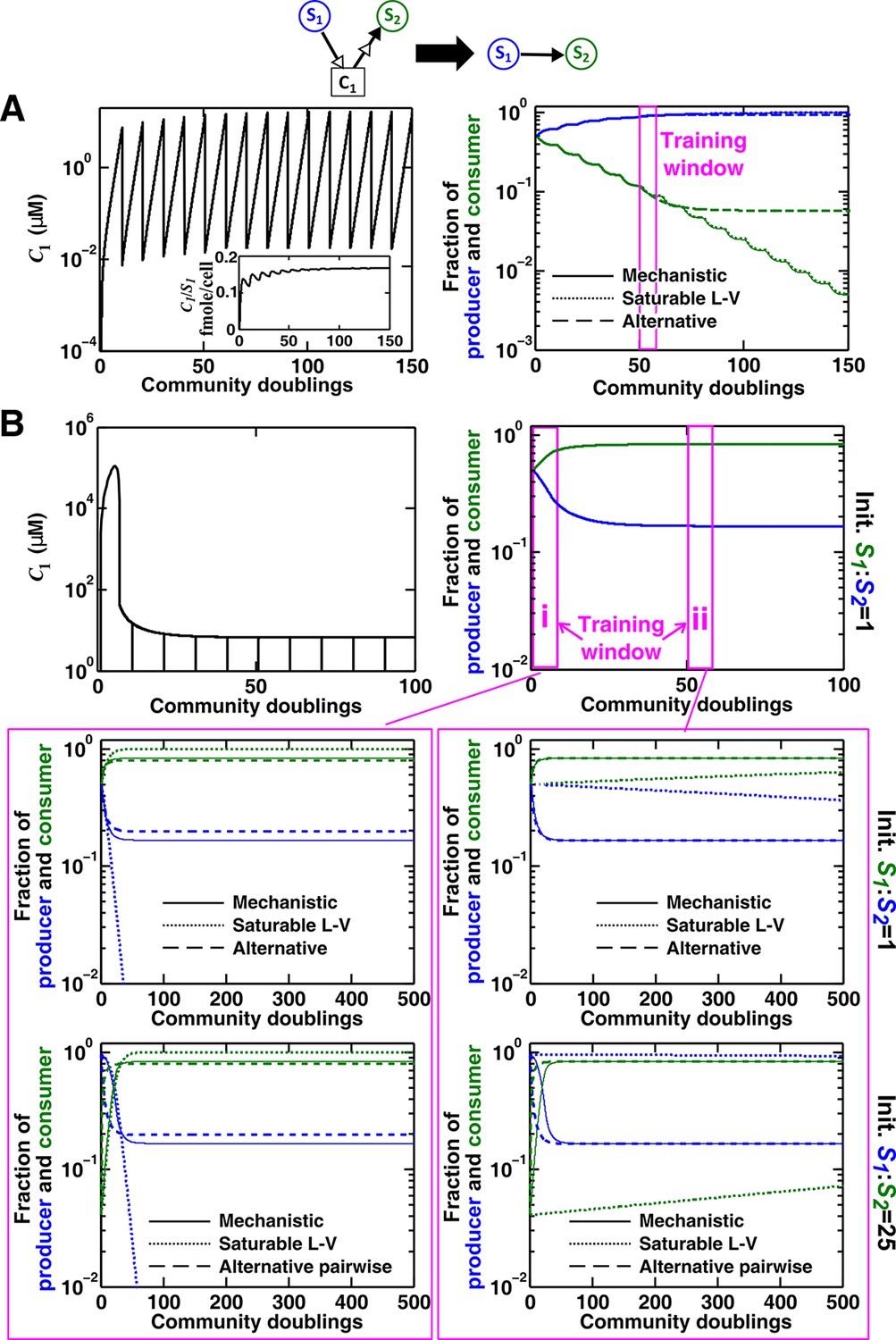
Saturable L-V and alternative pairwise models are not interchangeable.

Consider a commensal community with a consumable mediator C₁. (A) The mediator accumulates without reaching a steady state within each dilution cycle as the consumer S₂ gradually goes extinct (Figure 3B, Case I). After a few tens of generations, $C_{1}$ becomes proportional to its producer density $S_{1}$ (inset in left panel). In this case, a saturable L-V (dotted) but not the alternative pairwise model (dashed) is suitable. All parameters are listed in Figure 4—source data 1. (B) The consumable mediator reaches a non-zero steady state within each dilution cycle (Figure 3B, Case II). From mechanistic dynamics where initial species ratio is 1, we use two training windows to derive saturable L-V (dotted) and alternative (dashed) pairwise models. We then use these pairwise models to predict dynamics of communities starting at two different ratios. The alternative model but not the saturable L-V predicts the mechanistic model dynamics. All parameters are listed in Figure 4—source data 2. Note that in all figures, population fractions (instead of population densities) are plotted, which fluctuate less during dilutions compared to mediator concentration.

https://doi.org/10.7554/eLife.25051.017

Figure 4—source data 1 List of parameters for simulations in Figure 4 on an interaction through a reusable mediator.: https://doi.org/10.7554/eLife.25051.018
Download elife-25051-fig4-data1-v3.docx
Figure 4—source data 2 List of parameters for simulations in Figure 4 on an interaction through a consumable mediator.: https://doi.org/10.7554/eLife.25051.019
Download elife-25051-fig4-data2-v3.docx

Case II: When S₁ and S₂ can coexist (the basal fitness of S₁ is higher than the basal fitness of S₂ but less than the maximal fitness of S₂), a steady state solution for $C_{1}$ and species ratio $R_{S} = S_{2} / S_{1}$ exists (Figure 4B; Methods-Deriving a pairwise model for interactions mediated by a single consumable mediator Case II, Equation 11). To arrive at a pairwise model, we will need to eliminate $C_{1}$ which is mathematically possible (i.e. after community dynamics converges to the ‘ $f$ -zero-isocline’ on the phase plane of mediator $C_{1}$ and species ratio $R_{S}$ , as depicted by blue lines in Figure 3—figure supplement 2A–D). However, the derived pairwise model differs from the saturable L-V model:

\frac{d S_{2}}{d t} = r_{20} S_{2} + \frac{r_{S_{2} C_{1}} S_{1}}{ω S_{1} + ψ S_{2}} S_{2}

where constants $r_{20}$ , $r_{S_{2} C_{1}}$ , and $ω = 1 - K_{S_{2} C_{1}} / K_{C_{1} S_{2}}$ can be positive, negative, or zero, and ψ = $(K_{S_{2} C_{1}} α_{C_{1} S_{2}}) / (K_{C_{1} S_{2}} β_{C_{1} S_{1}})$ is positive (see Figure 1 table for parameter definitions and see Equation 13 in Methods). We will refer to this equation as ‘alternative pairwise model’, although the fitness influence term is a function of both $S_{1}$ and $S_{2}$ instead of the influencer $S_{1}$ alone as defined in the traditional L-V pairwise model.

Case III: When supplier S₁ always grows slower than consumer S₂, i.e. when the basal fitness of S₁ ( $r_{10}$ ) is less than the basal fitness of S₂ ( $r_{20}$ ), consumable $C_{1}$ declines to zero concentration. This is because C₁ is consumed by S₂ whose relative abundance over S₁ eventually exponentially increases at a rate of $r_{20} - r_{10}$ . Similar to Case II, under certain conditions (i.e. after community dynamics converges to the $f$ -zero-isocline as seen in Figure 3—figure supplement 2E–H), the alternative pairwise model (Equation 4) can be derived (Methods-Deriving a pairwise model for interactions mediated by a single consumable mediator, Case III).

For both Case II and Case III, we analytically demonstrate that in the absence of dilutions, alternative pairwise model dynamics can converge to mechanistic model dynamics (see Figure 3—figure supplements 3 and 5 for initial condition requirement and time scale of convergence). However, if initial $S_{1}$ and $S_{2}$ are such that the time scale of convergence is long compared to the duration of one dilution cycle (e.g. Figure 3—figure supplement 2C and G), then we will have to perform dilutions and the saturable L-V model can sometimes be more appropriate than the alternative model (Figure 3—figure supplement 4). Thus in these cases, whether a saturable L-V or an alternative model is more appropriate also depends on initial conditions.

The alternative model (Equation 4) can be further simplified to

d S_{2} / d t = (r_{20} + ρ S_{1} / S_{2}) S_{2}

if additionally, the half-saturation constant $K$ for C₁ consumption ( $K_{C_{1} S_{2}}$ ) is identical to that for C₁’s influence on the growth of consumer ( $K_{S_{2} C_{1}}$ ), and if S₂ has not gone extinct. This equation form has precedence in the literature (e.g. [Mougi and Kondoh, 2012]), where the interaction strength $r_{21}$ reflects the fact that the consumable mediator from $S_{1}$ is divided among consumer $S_{2}$ . Thus, we can regard the alternative model (Equation 4) or its simplified version (Equation 5) as a ‘divided influence’ model.

The saturable L-V model and the alternative model are not interchangeable (Figure 4). When a consumable mediator accumulates without reaching a steady state within each dilution cycle (Figure 4A left; inset: $C_{1}$ eventually becomes proportional to $S_{1}$ ), the saturable L-V model is predictive of community dynamics (Figure 4A right, compare dotted and solid lines). In contrast, predictions from the alternative pairwise model are qualitatively wrong (Figure 4A right, compare dashed and solid lines). When a consumable mediator eventually reaches a non-zero steady state within each dilution cycle (Figure 4B, black), could a saturable L-V model still work? The saturable L-V model derived from training window i (initial 10 generations) fails to predict species coexistence regardless of initial species ratios (Figure 4B left magenta box, compare solid with dotted). In comparison, the saturable L-V model derived from training window ii (at steady-state species ratio) performs better, especially if the starting species ratio is identical to that of the training dynamics (Figure 4B, top panel in right magenta box). However, at a different starting species ratio, the saturable L-V model fails to predict which species dominates the community (Figure 4B, bottom panel in right magenta box). In contrast, community dynamics can be described by the alternative pairwise model derived from either window i or ii (Figure 4B, compare dashed and solid lines in left and right magenta boxes).

We have shown here that even when one species affects another species via a single mediator, either a saturable L-V model or an alternative pairwise model may be appropriate. The appropriate model depends on whether the mediator is reusable or consumable, how fitness of the two species compare, and initial species densities (Figure 3; Figure 3—figure supplements 2–5). Choosing the wrong pairwise model generates qualitatively flawed predictions (Figure 4). Considering that reusable and consumable mediators are both common in microbial interactions, our results call for revisiting the universality assumption of pairwise modeling.

Two-mediator interactions require pairwise models different from single-mediator interactions

A species often affects another species via multiple mediators (Kato et al., 2008; Yang et al., 2009; Traxler et al., 2013; Kim et al., 2013). For example, a fraction of a population might die and release numerous chemicals, and some of these chemicals can simultaneously affect another individual. Here we examine the case where S₁ releases two reusable chemicals C₁ and C₂, both affecting the growth of S₂ (Figure 5A). Since the effect of each mediator can be described by a saturable L-V pairwise model (Figure 3A), we ask when the two mediators can be mathematically regarded as one mediator and described by a saturable L-V pairwise model (Figure 5B).

Figure 5 with 1 supplement see all

Download asset Open asset

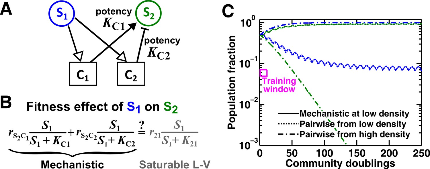
An example of a two-mediator interaction where a saturable L-V pairwise model may succeed or fail depending on initial conditions.

(A) One species can affect another species via two reusable mediators, each with a different potency $K_{C i}$ where $K_{C i}$ is $K_{S_{2} C_{i}} r_{10} / β_{C_{i} S_{1}}$ (Methods-Conditions under which a saturable L-V pairwise model can represent one species influencing another via two reusable mediators). A low $K_{C i}$ indicates a strong potency (e.g. high release of **C_i** by S₁ or low $C_{i}$ required to achieve half-maximal influence on S₂). (B) Under what conditions can an interaction via two reusable mediators with saturable effects on recipients be approximated by a saturable L-V pairwise model? (C) A community where the success or failure of a saturable L-V pairwise model depends on initial conditions. Here, $K_{C 1}$ = 10³ cells/ml and $K_{C 2}$ = 10⁵ cells/ml. Community dynamics starting at low $S_{1}$ (solid) can be predicted if the saturable L-V pairwise model is derived from reference dynamics starting at low (dotted). However, if we use a saturable L-V pairwise model derived from a community with high initial $S_{1}$ , prediction is qualitatively wrong (dash dot line). See Figure 5—figure supplement 1D for an explanation why a saturable L-V pairwise model estimated at one community density may not be applicable to another community density. Simulation parameters are listed in Figure 5—source data 1 .

https://doi.org/10.7554/eLife.25051.020

Figure 5—source data 1 List of parameters for simulations in Figure 5 on an interaction through two concurrent mediators.: https://doi.org/10.7554/eLife.25051.021
Download elife-25051-fig5-data1-v3.docx
Figure 5—source data 2 List of parameters for simulations in Figure 5—figure supplement 1 on an interaction through two concurrent mediators, assessed at high versus low cell densities.: https://doi.org/10.7554/eLife.25051.022
Download elife-25051-fig5-data2-v3.docx

We assume that fitness effects from different chemical mediators on a focal species are additive. Not making this assumption will likely violate the additivity assumption essential to pairwise models. Additive fitness effects have been observed for certain ‘homologous’ metabolites. For example, in multi-substrate carbon-limited chemostats of E. coli, the fitness effects from glucose and galactose were additive (Lendenmann and Egli, 1998). ‘Heterologous’ metabolites such as carbon and nitrogen sources likely affect cell fitness in a multiplicative fashion. However, if $W_{C}$ and $W_{N}$ , the fitness influences of released carbon and nitrogen with respect to those already in the environment, are both small (i.e. $W_{C}$ , $W_{N}$ < < 1), the additional relative fitness influence will be additive: $(1 + W_{C}) (1 + W_{N}) - 1 \approx W_{C} + W_{N}$ . However, we need to keep in mind that even among homologous metabolites, fitness effects may not be additive (Hermsen et al., 2015). ‘Sequential’ metabolites (e.g. diauxic shift) provide another example of non-additivity. Similar to the previous section, we assume that all abiotic resources are unlimited.

For the two reusable mediators, depending on their relative ‘potency’ (defined in Figure 5A legend), their combined effect generally cannot be modeled as a single mediator except under special conditions (Methods-Conditions under which a saturable L-V pairwise model can represent one species influencing another via two reusable mediators). These special conditions include: (1) mediators share similar potency (Figure 5—figure supplement 1B), or (2) one mediator dominates the interaction (Figure 5—figure supplement 1C). If these conditions are not satisfied, we can easily find examples where saturable L-V pairwise models derived from a low-density community and from a high-density community have qualitatively different parameters (Figure 5—figure supplement 1D). Consequently, the future dynamics of a low-density community can be predicted by a saturable L-V model derived from a low-density community but not by a model derived from a high-density community (Figure 5C). Thus, even though each mediator can be modeled by saturable L-V, their joint effects may or may not be modeled by saturable L-V depending on the relative potencies of the two mediators and sometimes even on initial conditions (high or low initial $S_{1}$ ).

Similarly, when both mediators are consumable and do not accumulate (as in Cases II and III of Figure 3B), the fitness effect term becomes $\frac{r_{S_{2} C_{1}} S_{1}}{ω_{C_{1}} S_{1} + ψ_{C_{1}} S_{2}} + \frac{r_{S_{2} C_{2}} S_{1}}{ω_{C_{2}} S_{1} + ψ_{C_{2}} S_{2}}$ . Except under special conditions (e.g. when $ω_{C_{1}}$ and $ω_{C_{2}}$ are zero, or when $ω_{C_{1}} / ω_{C_{2}} = ψ_{C_{1}} / ψ_{C_{2}}$ , or when one mediator dominates the interaction), the two mediators may not be regarded as one. By the same token, when one mediator is a steady-state consumable and the other is reusable, they generally may not be regarded as a single mediator and would require yet a different pairwise model (i.e. with the fitness effect term $\frac{r_{S_{2} C_{1}} S_{1}}{ω_{C_{1}} S_{1} + ψ_{C_{1}} S_{2}} + \frac{r_{S_{2} C_{2}} S_{1}}{S_{1} + K_{S_{2} C_{2}} r_{10} / β_{C_{2} S_{1}}}$ ).

In summary, when S₁ influences S₂ through multiple mediators, rarely can we approximate them as a single mediator. Sometimes, a pairwise model derived from one community may not apply to communities initiated at different densities (Figure 5C; Figure 5—figure supplement 1D). This casts further doubt on the usefulness of a single pairwise model for all pairwise microbial interactions.

L-V competition model can fail if two competing species engage in an additional interaction

So far, by assuming that abiotic resources are always present in excess (e.g. in turbidostats), we have not considered species competition for abiotic resources. In this section, we consider a competitive commensal community in a batch environment where S₁ and S₂ compete for an essential shared resource C₁ supplied by the environment at a constant rate (e.g. constant light), and S₁ supplies an essential consumable metabolite C₂ to promote S₂ growth (Figure 6A, left). We show that an L-V pairwise model works for some but not all communities even though these communities qualitatively share the same interaction mechanism.

Figure 6

Download asset Open asset

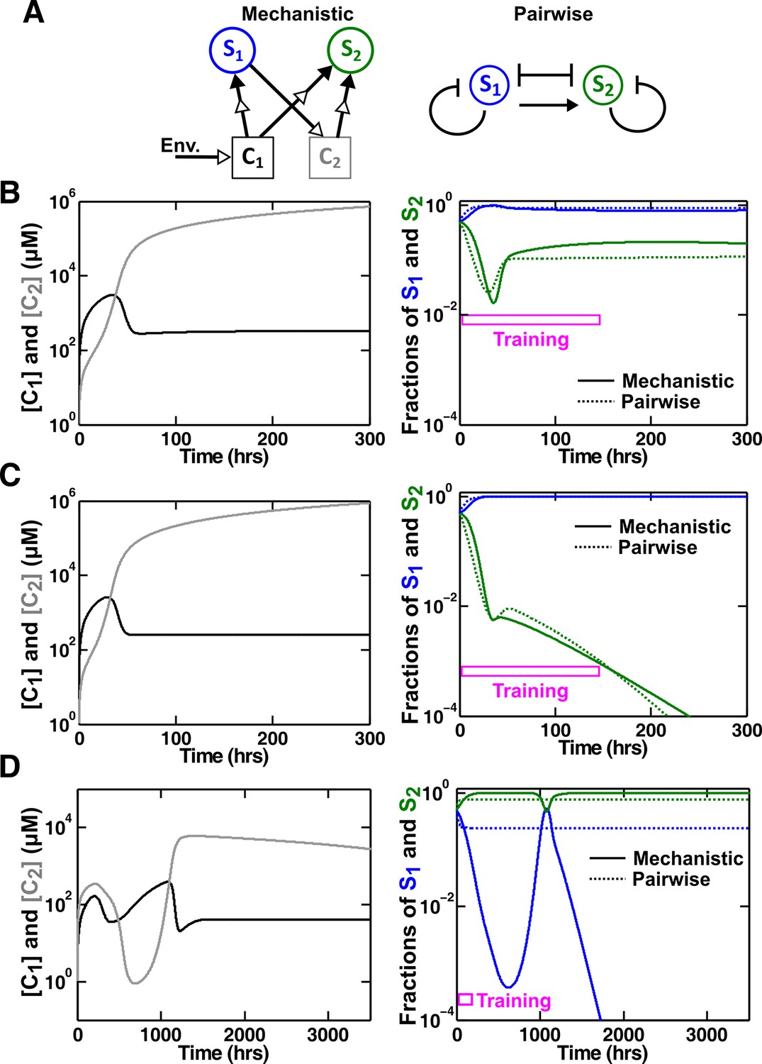
An example of a competitive commensal community where an L-V pairwise model may work or fail.

(A) Left: Two species S₁ and S₂ compete for shared resource C₁. Additionally, S₁ produces C₂ that promotes the growth of S₂ upon consumption. Right: An L-V pairwise model captures the intra- and inter-species competition as well as the commensal interaction between the two species. (B,C) Examples where L-V pairwise models predict the mechanistic reference dynamics well. (D) An example where the L-V pairwise model fails to predict the dynamics qualitatively (note the much longer time range). Here, population fractions fluctuate due to changes in relative concentration of C₁ compared to C₂. In all cases, the pairwise model is derived from the population dynamics in the initial stages of growth (150 hr in all cases). Simulation parameters are listed in Figure 6—source data 1.

https://doi.org/10.7554/eLife.25051.024

Figure 6—source data 1 List of parameters for simulations in Figure 6 on an interaction through a consumable mediator, for species consuming a shared abiotic resource.: https://doi.org/10.7554/eLife.25051.025
Download elife-25051-fig6-data1-v3.docx

In our mechanistic model (Methods-Competitive commensal interaction, Equation 47), the fitness of S₂ is multiplicatively affected by C₁ and C₂ (Mankad and Bungay, 1988). We choose parameters such that the effect from C₂ to S₂ is far from saturation (e.g. linear with respect to $C_{2}$ and $S_{1}$ ) to simplify the problem. In our L-V pairwise model (Figure 6A, right; Methods-Competitive commensal interaction, Equation 48), intra- and inter-species competition is represented by the traditional logistic L-V model (Equation 2; Gause, 1934; Thébault and Fontaine, 2010; Mougi and Kondoh, 2012). We then introduce a linear term ( $r_{21} S_{1}$ ) to describe the fitness effect of commensal interaction.

We tested various sets of mechanistic model parameters where the two species coexist in a steady fashion (Figure 6B), or one species goes extinct (Figure 6C), or species composition fluctuates (Figure 6D). L-V pairwise models deduced from a fixed period of training time could predict future dynamics in the first two cases, but failed to do so in the third case. Thus, depending on dynamic details of communities, a pairwise model sometimes works and sometimes fails.

To summarize our work, even for pairwise microbial interactions, depending on interaction mechanisms (reusable versus consumable mediator, single mediator versus multiple mediators), we will need to use a plethora of pairwise models to avoid qualitative failures in predicting which species dominates a community or whether species coexist (Figures 3, 4 and 5). Sometimes, even when different communities share identical interaction mechanisms, depending on details such as relative species fitness, interaction strength, and initial conditions, the best-fitting pairwise model may or may not predict future dynamics (Figure 3B, Figure 3—figure supplement 4, Figure 4, Figure 5, Figure 5—figure supplement 1, and Figure 6). This defeats the very purpose of pairwise modeling – using a single equation form to capture fitness effects of all pairwise species interactions regardless of interaction mechanisms or quantitative details. In a community of more than two microbial species, interaction modification can cause pairwise models to fail (Figure 7). Even if species interact in an interaction chain and thus interaction modification does not occur, various chain segments may require different forms of pairwise models. Taken together, a pairwise model is unlikely to be effective for predicting community dynamics especially if interaction mechanisms are diverse.

Figure 7 with 1 supplement see all

Download asset Open asset

Interaction chain but not interaction modification may be represented by a multispecies pairwise model.

We examine three-species communities engaging in indirect interactions. Each species pair is representable by a two-species pairwise model (saturable L-V or alternative pairwise model, purple in the right columns of B, D, and F). We then use these two-species pairwise models to construct a three-species pairwise model, and test how well it predicts the dynamics known from the mechanistic model. In B, D, and F, left panels show dynamics from the mechanistic models (solid lines) and three-species pairwise models (dotted lines). Right panels show the difference metric $\bar{D}$ . (**A–B**) Interaction chain: S₁ affects S₂, and S₂ affects S₃. The two interactions employ independent mediators C₁ and C₂, and both interactions can be represented by the saturable L-V pairwise model. The three-species pairwise model matches the mechanistic model in this case. Simulation parameters are provided in Figure 7—source data 1. (**C–F**) Interaction modification. In both cases, the three-species pairwise model fails to predict reference dynamics even though the dynamics of each species pair can be represented by a pairwise model. (**C–D**) S₃ consumes C₁, a mediator by which S₁ stimulates S₂. Parameters are listed in Figure 7—source data 2. Here, S₁ changes the nature of interaction between S₂ and **S₃: S₂** and S₃ do not interact in the absence of S₁, but S₃ inhibits S₂ in the presence of S₁. The three-species pairwise model makes qualitatively wrong prediction about species coexistence. As expected, if S₃ does not remove C₁, the three-species pairwise model works (Figure 7—figure supplement 1A–B). (**E–F**) S₁ and S₃ both supply C₁ which stimulates S₂. Here, no species changes ‘the nature of interactions’ between any other two species: both S₁ and S₃ contribute reusable C₁ to stimulate **S₂. S₁** promotes S₂ regardless of **S₃; S₃** promotes S₂ regardless of **S₁; S₁** and S₃ do not interact regardless of S₂. However, a multispecies pairwise model assumes that the fitness effects from the two producers on S₂ will be additive, whereas in reality, the fitness effect on S₂ saturates at high . As a result, the three-species pairwise model qualitatively fails to capture relative species abundance. As expected, if C₁ affects S₂ in a linear fashion, the community dynamics is accurately captured in the multispecies pairwise model (Figure 7—figure supplement 1C–D). Simulation parameters are listed in Figure 7—source data 3.

https://doi.org/10.7554/eLife.25051.026

Figure 7—source data 1 List of parameters for simulations in Figure 7B on interaction between three species in a chain.: https://doi.org/10.7554/eLife.25051.027
Download elife-25051-fig7-data1-v3.docx
Figure 7—source data 2 List of parameters for simulations in Figure 7D on interaction modification through consumption of a shared mediator by a third species.: https://doi.org/10.7554/eLife.25051.028
Download elife-25051-fig7-data2-v3.docx
Figure 7—source data 3 List of parameters for simulations in Figure 7F on interaction modification through production of a shared mediator by a third species.: https://doi.org/10.7554/eLife.25051.029
Download elife-25051-fig7-data3-v3.docx
Figure 7—source data 4 List of parameters for simulations in Figure 7—figure supplement 1B on an interaction between three species through a shared reusable mediator affecting multiple species.: https://doi.org/10.7554/eLife.25051.030
Download elife-25051-fig7-data4-v3.docx
Figure 7—source data 5 List of parameters for simulations in Figure 7—figure supplement 1D on an interaction between three species through a shared reusable mediator produced by multiple species.: https://doi.org/10.7554/eLife.25051.031
Download elife-25051-fig7-data5-v3.docx

Discussions

Multispecies pairwise models are widely used in theoretical ecology due to their simplicity. These models assume that all pairwise species interactions can be captured by a single pairwise model regardless of interaction mechanisms or quantitative details of a community (universality assumption). This assumption may be satisfied if, for example, interaction mediators are always species themselves (e.g. prey-predation in a food web) so that pairwise models are equivalent to mechanistic models. However, interactions in microbial communities are diverse and often mediated by chemicals (Figure 2). Here, we consider the validity of universality assumption of pairwise models in well-mixed, two-species microbial communities. We have focused on various types of chemical-mediated interactions commonly encountered in microbial communities (Figure 2) (Kato et al., 2005; Gause, 1934; Ghuysen, 1991; Jakubovics et al., 2008; Chen et al., 2004; D'Onofrio et al., 2010; Johnson et al., 1982; Hamilton and Ng, 1983). For each type of species interaction, we construct a mechanistic model to generate reference community dynamics (akin to experimental results). We then attempt to derive the best-matching pairwise model and ask how predictive it is.

We first consider cases where abiotic resources are in excess. When one species affects another species via a single chemical mediator, either the saturable L-V or the alternative pairwise model is appropriate, depending on the interaction mechanism (consumable versus reusable mediator), relative fitness of the two species, and initial conditions (Figure 3; Figure 3—figure supplement 2 to Figure 3—figure supplement 5). These two models are not interchangeable (Figure 4). If one species influences another species through multiple mediators, then in general, these mediators may not be regarded as a single mediator nor representable by a single pairwise model. For example, for two reusable mediators, unless their potencies are similar or one mediator is much more potent than the other, saturable L-V model parameters can qualitatively differ depending on initial community density (Figure 5—figure supplement 1D). Consequently, a pairwise model derived from a high-density community generates false predictions for low-density communities (Figure 5C), limiting the usefulness of pairwise models. We then consider a community where two species compete for a shared resource while engaging in commensalism via a single chemical mediator. We find that the best-fitting L-V pairwise model can predict future dynamics in some but not all communities, depending on parameters used in the mechanistic model (Figure 6). Thus, although a single equation form can work in many cases, it generates qualitatively wrong predictions in many other cases.

In communities of more than two microbial species, indirect interactions via a third species can occur. When indirect interactions take the form of interaction chains, if each chain segment of two species engages in an independent interaction and can be represented by a pairwise model, then multispecies pairwise models can work (Figure 7A-B). However, as discussed above, pairwise equation forms may vary among chain segments depending on interaction mechanisms and quantitative details of a community. When indirect interactions take the form of interaction modification, even if each species pair can be accurately represented by a pairwise model, a multispecies pairwise model may fail (Figure 7C–F, ). Interaction modification includes trait modification (Wootton, 2002; Werner and Peacor, 2003; Schmitz et al., 2004), or, in our cases, mediator modification. Mediator modification is very common in microbial communities. For example, antibiotic released by one species to inhibit another species may be inactivated by a third species, and this type of indirect interactions can stabilize microbial communities (Kelsic et al., 2015; Bairey et al., 2016). As another example, interaction mediators are often generated by and shared among multiple species. For example in oral biofilms, organic acids such as lactic acid are generated from carbohydrate fermentation by many species (Bradshaw et al., 1994; Marsh and Bradshaw, 1997; Kuramitsu et al., 2007). Such by-products are also consumed by multiple species (Kolenbrander, 2000).

One can argue that an extended pairwise model (e.g. $\frac{d S_{2}}{d t} = r_{20} S_{2} + \frac{r_{S_{2} C} S_{1}}{ς + ω S_{1} + ψ S_{2}} S_{2}$ ) embodying both the saturable form and the alternative form can serve as a general-purpose model at least for pairwise interactions via a single mediator. In fact, even the effects of indirect interactions may be quantified and included in the model by incorporating higher-order interaction terms (Case and Bender, 1981; Worthen and Moore, 1991), although with many challenges (Wootton, 2002). In the end, although these strategies may lead to a sufficiently accurate phenomenological model especially within the training window, they may fail to predict future dynamics.

When might a pairwise model be useful? First, pairwise models have been instrumental in understanding ecological phenomena such as prey-predator oscillatory dynamics and coexistence of competing predator species (Volterra, 1926; MacArthur, 1970; Case and Casten, 1979; Chesson, 1990). In these cases, mechanistic models are either identical to pairwise models or can be transformed into pairwise models under simplifying assumptions. Second, pairwise models of pairwise species interactions can provide a bird’s-eye view of strong or weak stimulatory or inhibitory interactions in a community. For example, Vetsigian et al., 2011 found that interactions between soil-isolated Streptomyces strains are enriched for reciprocity – if A inhibits or promotes B, it is likely that B also inhibits or promotes A (Vetsigian et al., 2011). Third, pairwise models have been useful in qualitatively understanding species assembly rules in small communities (Friedman et al., 2017). That is, qualitative information regarding species survival in competitions among a small number of species may be used to predict survival in more diverse communities within a similar time window. Fourth, a pairwise model can serve as a starting point for generating hypotheses on species interactions (e.g. Li et al., 2015). Note that when applied to microbial communities (Mounier et al., 2008; Stein et al., 2013; Marino et al., 2014), a fitting pairwise model means that the training dynamics of the community under investigation can be approximated by a theoretical community where species interactions satisfy the additivity and universality assumptions of pairwise models. Even though the theoretical community is likely different from the real community, hypothesis formulation can still be valuable. Finally, pairwise models can be useful in making predictions of limited scales. For example, Stein et al. used 2/3 of community dynamics data as a training set to derive a multispecies pairwise model, and in the best-case scenario, the model generated reasonable predictions on the remaining 1/3 of data (Stein et al., 2013). However, as we have shown, pairwise models can generate qualitatively wrong predictions (Figures 4–7), especially if interaction mechanisms are diverse such as in microbial communities. Not surprisingly, predicting qualitative consequences of species removal or addition using a pairwise model has encountered difficulties, especially in communities of more than three species (Mounier et al., 2008; Friedman et al., 2017).

An alternative to a pairwise model is a mechanistic model. How much information about interaction mechanisms do we need to construct a mechanistic model? That is, what is the proper level of abstraction which captures the phenomena of interest, yet avoids unnecessary details (Li et al., 2015; Durrett and Levin, 1994)? For example, Tilman argued that if a small number of mechanisms (e.g. the ‘axes of trade-offs’ in species traits) could explain much of the observed pattern (e.g. species coexistence), then this abstraction would be highly revealing (Tilman, 1987). However, the choice of abstraction is often not obvious. Consider for example a commensal community where S₁ grows exponentially (not explicitly depicted in equations in Figure 8) and the net growth rate of S₂, which is normally zero, is promoted by mediator C from S₁ in a linear fashion (Figure 8). If we do not know how S₁ stimulates S₂, we can still construct an L-V pairwise model (Figure 8A). If we know the identity of mediator C and realize that C is consumable, then we can instead construct a mechanistic model incorporating $C$ (Figure 8B). However, if C is produced from a precursor via an enzyme E released by S₁, then we get a different form of mechanistic model (Figure 8C). If, on the other hand, E is anchored on the membrane of S₁ and each cell expresses a similar amount of $E$ , then equations in Figure 8D are mathematically equivalent to Figure 8B. This simple example, inspired by extracellular breakdown of cellulose into a consumable sugar C (Bayer and Lamed, 1986; Felix and Ljungdahl, 1993; Schwarz, 2001), illustrates how knowledge of mechanisms may eventually help us determine the right level of abstraction.

Figure 8

Download asset Open asset

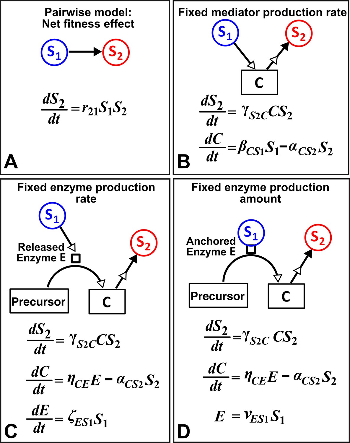
Different levels of abstraction in a mechanistic model.

How one species (S₁) may influence another (S₂) can be mechanistically modeled at different levels of abstraction. For simplicity, here we assume that interaction strength scales in a linear (instead of saturable) fashion with respect to mediator concentration or species density. The basal fitness of S₂ is zero. (A) In the simplest form, S₁ stimulates S₂ in an L-V pairwise model. (B) In a mechanistic model, we may realize that S₁ stimulates S₂ via a mediator C which is consumed by S₂. The corresponding mechanistic model is given. (C) Upon probing more deeply, it may become clear that S₁ stimulates S₂ via an enzyme E, where E degrades an abundant precursor (such as cellulose) to generate mediator C (such as glucose). In the corresponding mechanistic model, we may assume that E is released by S₁ at a rate $ζ_{E S 1}$ and that E liberates C at a rate $η_{C E}$ . (D) If instead E is anchored on the cell surface (e.g. cellulosome), then E is proportional to S₁. If we substitute E into the second equation, then (B) and (D) become equivalent. Thus, when enzyme is anchored on cell surface but not when enzyme is released, the mechanistic knowledge of enzyme can be neglected.

https://doi.org/10.7554/eLife.25051.033

In summary, under certain circumstances, we may already know that microbial interaction mechanisms fall within the domain of validity for a particular pairwise model. In these cases, a pairwise model provides the appropriate level of abstraction, and constructing such a pairwise model is much easier than a mechanistic model (Figure 1). However, if we do not know whether a pairwise model is valid, we will need to be cautious since pairwise models can fail to even qualitatively capture pairwise microbial interactions. We need to be equally careful when extrapolating and generalizing conclusions obtained from pairwise models, especially for communities where species interaction mechanisms are diverse. Considering recent advances in identifying and quantifying interactions, we advocate a transition to models that incorporate interaction mechanisms at the appropriate level of abstraction.

Materials and methods

Interaction modification but not interaction chain violates the additivity assumption

Request a detailed protocol

In a pairwise model, the fitness of a focal species S_i is the sum of its ‘basal fitness’ ( $r_{i 0}$ , the net growth rate of a single S_i individual in the absence of any intra-species or inter-species interactions) and the additive fitness effects exerted by pairwise interactions with other members of the community. Mathematically, an $N$ -species pairwise model is often formulated as

\frac{d S_{i}}{d t} = (r_{i 0} + \sum_{j = 1}^{N} f_{i j} (S_{j})) S_{i}

Here, $f_{i j} (S_{j})$ describes how $S_{j}$ , the density of species S_j, positively or negatively affects the fitness of S_i, and is a linear or nonlinear function of only $S_{j}$ .

Indirect interactions via a third species fall under two categories (Wootton, 1993). The first type is known as ‘interaction chain’ or ‘density-mediated indirect interactions’. For example, the consumption of plant S₁ by herbivore S₂ is reduced when the density of herbivore is reduced by carnivore S₃. In this case, the three-species pairwise model

{\begin{cases} \frac{d S_{1}}{d t} & = (r_{10} - f_{12} (S_{2})) S_{1} \\ \frac{d S_{2}}{d t} & = (r_{20} + f_{21} (S_{1}) - f_{23} (S_{3})) S_{2} \\ \frac{d S_{3}}{d t} & = (r_{30} + f_{32} (S_{2})) S_{3} \end{cases}

does not violate the additivity assumption (compare with Equation 6 (Case and Bender, 1981; Wootton, 1994).

The second type of indirect interactions is known as ‘interaction modification’ or ‘trait-mediated indirect interactions’ or ‘higher order interactions’ (Vandermeer, 1969; Wootton, 1994; Billick and Case, 1994; Wootton, 2002), where a third species modifies the ‘nature of interaction’ from one species to another (Wootton, 2002; Werner and Peacor, 2003; Schmitz et al., 2004). For example, when carnivore is present, herbivore will spend less time foraging and consequently plant density increases. In this case, $f_{12}$ in Equation 7 is a function of both $S_{2}$ and $S_{3}$ , violating the additivity assumption.

Summary of simulation files

Request a detailed protocol

Simulations are based on Matlab and executed on an ordinary PC. Steps are:

Step 1: Identify monoculture parameters $r_{i 0}$ , $r_{i i}$ , and $K_{i i}$ (Figure 1—figure supplement 2C, Row 1 and Row 2).

Step 2: Identify interaction parameters $r_{i j}$ , $r_{j i}$ , $K_{i j}$ , and $K_{j i}$ where $i \neq j$ (Figure 1—figure supplement 2C, Row 3).

Step 3: Calculate distance $\bar{D}$ between population dynamics of the reference mechanistic model and the approximate pairwise model over a period of time outside of the training window to assess if the pairwise model is predictive.

Fitting is performed using nonlinear least squares (lsqnonlin routine) with default optimization parameters. The following list describes the m-files used for different steps of the analysis:

File name	Function
FitCost_BasalFitness Source code 1	Calculates the cost function for monocultures (i.e. the difference between the target mechanistic model dynamics and the dynamics obtained from the pairwise model)
FitCost_BFSatLV.m Source code 2	Calculates the cost function for communities (i.e. the difference between the target mechanistic model dynamics and the dynamics obtained from the saturable L-V pairwise model)
FitCost_BFSatLV_Dp.m Source code 3	Calculates the cost function for communities (i.e. the difference between the target mechanistic model dynamics and the dynamics obtained from the alternative pairwise model)
DynamicsMM_WM_MonocultureDpMM.m Source code 4	Returns growth dynamics for monocultures, based on the mechanistic model
DynamicsMMSS_WM_NetworkDpMM.m Source code 5	Returns growth dynamics for communities of multiple species, based on the mechanistic model
DynamicsWM_NetworkBFSatLV.m Source code 6	Returns growth dynamics for communities of multiple species, based on the saturable L-V pairwise model
DynamicsWM_NetworkBFSatLV_Dp.m Source code 7	Returns growth dynamics for communities of multiple species, based on the alternative pairwise model
DeriveBasalFitnessMM_WM_DpMM.m Source code 8	Estimates monoculture parameters of pairwise model (Step 1)
DeriveBFSatLVMMSS_WM_DpMM.m Source code 9	Estimates saturable L-V pairwise model interaction parameters (Step 2)
DeriveBFSatLVMMSS_WM_DpMM_Dp.m Source code 10	Estimates alternative pairwise model interaction parameters (Step 2)
DeriveBFSatLVMMSS_WM_DpMM_r21.m Source code 11	Estimates saturable L-V pairwise model interaction parameters ( $r_{21}$ and $K_{21}$ ) in cases where we know that S₂ is only affected by S₁, to accelerate optimization
DeriveBFSatLVMM_WM_DpMM_Dp_r21.m Source code 12	Estimates alternative pairwise model interaction parameter ( $r_{21}$ ) in cases where we know that S₂ is only affected by S₁ and that $K_{S 2 C 1} = K_{C 1 S 2}$ to accelerate optimization
DynamicsWM_NetworkBFLogLV_DI.m Source code 13	Returns growth dynamics for communities of two species competing for an environmental resource while engaging in an additional interaction, based on the logistic L-V pairwise model (Figure 6)
C2Sp2_ARCLi_NoSatDp_FitBFLogLV_DI.m Source code 14	Estimates logistic L-V pairwise model interaction parameters for communities of two species competing for an environmental resource while engaging in an additional interaction, and compares community dynamics from pairwise and mechanistic models (Figure 6)
Dynamics_WM_NetworkDpMM_ODE23.m Source code 15	Defines differential equations when using Matlab’s ODE23 solver to calculate community dynamics
Case_C1Sp2_CmnsDp_ODE23.m Source code 16	Example of using Matlab ODE23 solver for calculating community dynamics

File name

Function

FitCost_BasalFitness

Source code 1

Calculates the cost function for monocultures (i.e. the difference between the target mechanistic

model dynamics and the dynamics obtained from the pairwise model)

FitCost_BFSatLV.m

Source code 2

Calculates the cost function for communities (i.e. the difference between the target mechanistic

model dynamics and the dynamics obtained from the saturable L-V pairwise model)

FitCost_BFSatLV_Dp.m

Source code 3

Calculates the cost function for communities (i.e. the difference between the target mechanistic model

dynamics and the dynamics obtained from the alternative pairwise model)

DynamicsMM_WM_MonocultureDpMM.m

Source code 4

Returns growth dynamics for monocultures, based on the mechanistic model

DynamicsMMSS_WM_NetworkDpMM.m

Source code 5

Returns growth dynamics for communities of multiple species, based on the mechanistic model

DynamicsWM_NetworkBFSatLV.m

Source code 6

Returns growth dynamics for communities of multiple species, based on the saturable L-V pairwise

model

DynamicsWM_NetworkBFSatLV_Dp.m

Source code 7

Returns growth dynamics for communities of multiple species, based on the alternative pairwise model

DeriveBasalFitnessMM_WM_DpMM.m

Source code 8

Estimates monoculture parameters of pairwise model (Step 1)

DeriveBFSatLVMMSS_WM_DpMM.m

Source code 9

Estimates saturable L-V pairwise model interaction parameters (Step 2)

DeriveBFSatLVMMSS_WM_DpMM_Dp.m

Source code 10

Estimates alternative pairwise model interaction parameters (Step 2)

DeriveBFSatLVMMSS_WM_DpMM_r21.m

Source code 11

Estimates saturable L-V pairwise model interaction parameters ( $r_{21}$ and $K_{21}$ ) in cases where we know

that S₂ is only affected by S₁, to accelerate optimization

DeriveBFSatLVMM_WM_DpMM_Dp_r21.m

Source code 12

Estimates alternative pairwise model interaction parameter ( $r_{21}$ ) in cases where we know that S₂

is only affected by S₁ and that $K_{S 2 C 1} = K_{C 1 S 2}$ to accelerate optimization

DynamicsWM_NetworkBFLogLV_DI.m

Source code 13

Returns growth dynamics for communities of two species competing for an environmental resource

while engaging in an additional interaction, based on the logistic L-V pairwise model (Figure 6)

C2Sp2_ARCLi_NoSatDp_FitBFLogLV_DI.m

Source code 14

Estimates logistic L-V pairwise model interaction parameters for communities of two species

competing for an environmental resource while engaging in an additional interaction, and

compares community dynamics from pairwise and mechanistic models (Figure 6)

Dynamics_WM_NetworkDpMM_ODE23.m

Source code 15

Defines differential equations when using Matlab’s ODE23 solver to calculate community dynamics

Case_C1Sp2_CmnsDp_ODE23.m

Source code 16

Example of using Matlab ODE23 solver for calculating community dynamics

Deriving a pairwise model for interactions mediated by a single consumable mediator

To facilitate mathematical analysis, we assume that requirements calculated below are eventually satisfied within each dilution cycle (see Figure 3—figure supplement 4 for an example where dilution cycles necessitated by long convergence time violate requirements for a pairwise model to converge to the mechanistic model). We further assume that $r_{10} > 0$ and $r_{20} > 0$ so that species cannot go extinct in the absence of dilution. See Figure 3—figure supplement 5 for a summary of this section.

When S₁ releases a consumable mediator which stimulates the growth of S₂, the mechanistic model as per Figure 3B, is

{\begin{cases} \frac{d S_{1}}{d t} & = r_{10} S_{1} \\ \frac{d S_{2}}{d t} & = r_{20} S_{2} + r_{S_{2} C_{1}} \frac{C_{1}}{C_{1} + K_{S_{2} C_{1}}} S_{2} \\ \frac{d C_{1}}{d t} & = β_{C_{1} S_{1}} S_{1} - α_{C_{1} S_{2}} \frac{C_{1}}{C_{1} + K_{C_{1} S_{2}}} S_{2} = (β_{C_{1} S_{1}} - α_{C_{1} S_{2}} \frac{C_{1}}{C_{1} + K_{C_{1} S_{2}}} \frac{S_{2}}{S_{1}}) S_{1} \end{cases}

Let $C_{1} (t = 0) = C_{10} = 0$ ; $S_{1} (t = 0) = S_{10}$ ; and $S_{2} (t = 0) = S_{20}$ . Note that the initial condition $C_{10} = 0$ can be easily imposed experimentally by pre-washing cells. Under which conditions can we eliminate $C_{1}$ so that we can obtain a pairwise model of $S_{1}$ and $S_{2}$ ?

Define $R_{S} = S_{2} / S_{1}$ as the ratio of the two populations.

\begin{matrix} \frac{d R_{S}}{d t} = \frac{\frac{d S_{2}}{d t} S_{1} - S_{2} \frac{d S_{1}}{d t}}{S_{1}^{2}} = (r_{20} + r_{S_{2} C_{1}} \frac{C_{1}}{C_{1} + K_{S_{2} C_{1}}}) \frac{S_{2}}{S_{1}} - \frac{S_{2}}{S_{1}^{2}} r_{10} S_{1} \\ = (r_{20} + r_{S_{2} C_{1}} \frac{C_{1}}{C_{1} + K_{S_{2} C_{1}}} - r_{10}) R_{S} \end{matrix}

Case I: $r_{10} - r_{20} > r_{S_{2} C_{1}}$

Request a detailed protocol

Since producer S₁ always grows faster than consumer S₂, $R_{S} \to 0$ as $t \to \infty$ . Define ${\tilde{C}}_{1} = C_{1} / S_{1}$ (‘~' indicating scaling against a function).

\begin{matrix} \frac{d \tilde{C_{1}}}{d t} = \frac{d (C_{1} / S_{1})}{d t} = \frac{\frac{d C_{1}}{d t} S_{1} - C_{1} \frac{d S_{1}}{d t}}{S_{1}^{2}} = \frac{(β_{C_{1} S_{1}} S_{1} - \frac{α_{C_{1} S_{2}} C_{1}}{C_{1} + K_{C_{1} S_{2}}} S_{2}) S_{1} - C_{1} r_{10} S_{1}}{S_{1}^{2}} \\ = β_{C_{1} S_{1}} - r_{10} \tilde{C_{1}} - \frac{α_{C_{1} S_{2}} {\tilde{C}}_{1}}{{\tilde{C}}_{1} + K_{C_{1} S_{2}} \exp (- r_{10} t) / S_{10}} R_{S} \end{matrix}

Since $R_{S}$ declines exponentially with a rate faster than $| r_{20} + r_{S_{2} C_{1}} - r_{10} |$ , we can ignore the third term of the right hand side of Equation 10 if it is much smaller than the first term. That is,

\frac{α_{C_{1} S_{2}} {\tilde{C}}_{1}}{{\tilde{C}}_{1} + K_{C_{1} S_{2}} \exp (- r_{10} t) / S_{10}} R_{S} < α_{C_{1} S_{2}} R_{S} \leq α_{C_{1} S_{2}} R_{S} (0) \exp (- | r_{20} + r_{S_{2} C_{1}} - r_{10} | t) ≪ β_{C_{1} S_{1}} .

Thus for $t ≫ \ln (\frac{α_{C_{1} S_{2}} R_{S} (0)}{β_{C_{1} S_{1}}}) / | r_{20} + r_{S_{2} C_{1}} - r_{10} |$ , $\frac{d {\tilde{C}}_{1}}{d t} \approx β_{C_{1} S_{1}} - r_{10} {\tilde{C}}_{1}$ . When initial $\tilde{C_{1}}$ is 0, this equation can be solved to yield: $\tilde{C_{1}} \approx β_{C_{1} S_{1}} (1 - \exp (- r_{10} t)) / r_{10}$ . After time of the order of $1 / r_{10}$ , the second term can be neglected. Thus, $\tilde{C_{1}} \approx β_{C_{1} S_{1}} / r_{10}$ after time of the order of $max (\ln (\frac{α_{C_{1} S_{2}} R_{S} (0)}{β_{C_{1} S_{1}}}) / | r_{20} + r_{S_{2} C_{1}} - r_{10} |, 1 / r_{10})$ . Then $C_{1}$ can be replaced by $(β_{C_{1} S_{1}} / r_{10}) S_{1}$ in Equation 8, and a saturable L-V pairwise model can be derived.

Case II: $r_{S_{2} C_{1}} > r_{10} - r_{20} > 0$

Request a detailed protocol

For Equation 8, we find that a steady state solution for $C_{1}$ and $R_{S}$ , denoted respectively as $C_{1}^{*}$ and $R_{S}^{*}$ , exist. They can be easily found by setting the growth rates of S₁ and S₂ to be equal, and $d C_{1} / d t$ to zero.

{\begin{matrix} C_{1}^{*} = \frac{r_{10} - r_{20}}{r_{20} + r_{S_{2} C_{1}} - r_{10}} K_{S_{2} C_{1}} \\ R_{S}^{*} = \frac{β_{C_{1} S_{1}}}{α_{C_{1} S_{2}}} (1 + \frac{K_{C_{1} S_{2}}}{C_{1}^{*}}) \end{matrix}

However, if $C_{1}$ has not yet reached steady state, imposing steady state assumption would falsely predict $R_{S}$ at steady state and thus remaining at its initial value (Figure 4Bii , dotted lines). Since $d C_{1} / d t$ in Equation 8 is the difference between two exponentially growing terms, we factor out the exponential term $S_{1}$ to obtain

\frac{d C_{1}}{d t} = (β_{C_{1} S_{1}} - α_{C_{1} S_{2}} \frac{C_{1}}{C_{1} + K_{C_{1} S_{2}}} \frac{S_{2}}{S_{1}}) S_{1} = β_{C_{1} S_{1}} f (C_{1}, R_{S}) S_{1}

where $f (C_{1}, R_{S}) = 1 - \frac{α_{C_{1} S_{2}}}{β_{C_{1} S_{1}}} \frac{C_{1}}{C_{1} + K_{C_{1} S_{2}}} R_{S}$ . When $f \approx 0$ , we can eliminate $C_{1}$ and obtain an alternative pairwise model

\frac{d S_{2}}{d t} = r_{20} S_{2} + r_{S_{2} C_{1}} \frac{β_{C_{1} S_{1}} K_{C_{1} S_{2}} S_{1}}{β_{C_{1} S_{1}} (K_{C_{1} S_{2}} - K_{S_{2} C_{1}}) S_{1} + α_{C_{1} S_{2}} K_{S_{2} C_{1}} S_{2}} S_{2}

\frac{d S_{2}}{d t} = r_{20} S_{2} + \frac{r_{S_{2} C_{1}} S_{1}}{ω S_{1} + ψ S_{2}} S_{2}

where ω and ψ are constants (Figure 3Bii).

For certain conditions (which will be discussed at the end of this section, Figure 3—figure supplement 5A), this alternative model can make reasonable predictions of community dynamics even before the community reaches the steady state (Figure 4Bii , compare dashed and solid lines). Below we discuss the general properties of community dynamics and show that there exists a time scale $t_{f}$ after which it is reasonable to assume $f \approx 0$ and the alternative model can be derived. We also estimate $t_{f}$ for several scenarios.

We first make $C_{1}$ and $R_{S}$ dimensionless by defining ${\hat{C}}_{1} = C_{1} / C_{1}^{*}$ and ${\hat{R}}_{S} = R_{S} / R_{S}^{*}$ (‘ ^ ' indicating scaling against steady state values). Equation 9 can then be rewritten as

\frac{d {\hat{R}}_{S}}{d t} = (r_{20} + r_{S_{2} C_{1}} \frac{{\hat{C}}_{1}}{{\hat{C}}_{1} + {\hat{K}}_{S_{2} C_{1}}} - r_{10}) {\hat{R}}_{S}

where ${\hat{K}}_{S_{2} C_{1}} = K_{S_{2} C_{1}} / C_{1}^{*}$ .

From Equations 8 and 11, we obtain

\begin{array}{ll} \frac{d \frac{C_{1}}{C_{1}^{*}}}{d t} = \frac{1}{C_{1}^{*}} (β_{C_{1} S_{1}} - \frac{α_{C_{1} S_{2}} C_{1}}{C_{1} + K_{C_{1} S_{2}}} \frac{R_{S}}{R_{S}^{*}} R_{S}^{*}) S_{1} = \frac{1}{C_{1}^{*}} (β_{C_{1} S_{1}} - \frac{α_{C_{1} S_{2}} C_{1}}{C_{1} + K_{C_{1} S_{2}}} {\hat{R}}_{S} R_{S}^{*}) \end{array} S_{1} = \frac{1}{C_{1}^{*}} (β_{C_{1} S_{1}} - \frac{α_{C_{1} S_{2}} C_{1} / C_{1}^{*}}{C_{1} / C_{1}^{*} + K_{C_{1} S_{2}} / C_{1}^{*}} {\hat{R}}_{S} \frac{β_{C_{1} S_{1}}}{α_{C_{1} S_{2}}} (1 + \frac{K_{C_{1} S_{2}}}{C_{1}^{*}})) S_{1} = \frac{1}{C_{1}^{*}} β_{C_{1} S_{1}} (1 - \frac{{\hat{C}}_{1} (1 + {\hat{K}}_{C_{1} S_{2}})}{{\hat{C}}_{1} + {\hat{K}}_{C_{1} S_{2}}} {\hat{R}}_{S}) S_{1}

\frac{d {\hat{C}}_{1}}{d t} = {\hat{β}}_{C_{1} S_{1}} [1 - \frac{{\hat{C}}_{1} (1 + {\hat{K}}_{C_{1} S_{2}})}{{\hat{C}}_{1} + {\hat{K}}_{C_{1} S_{2}}} {\hat{R}}_{S}] S_{1}

where ${\hat{β}}_{C_{1} S_{1}} = β_{C_{1} S_{1}} / C_{1}^{*}$ and ${\hat{K}}_{C_{1} S_{2}} = K_{C_{1} S_{2}} / C_{1}^{*}$ .

Using these scaled variables, $f$ (i.e. the square bracket in Equation 15) can be rewritten as

f ({\hat{C}}_{1}, {\hat{R}}_{S}) = 1 - \frac{{\hat{C}}_{1} (1 + {\hat{K}}_{C_{1} S_{2}})}{{\hat{C}}_{1} + {\hat{K}}_{C_{1} S_{2}}} {\hat{R}}_{S}

and

\frac{d {\hat{C}}_{1}}{d t} = {\hat{β}}_{C_{1} S_{1}} f ({\hat{C}}_{1}, {\hat{R}}_{S}) S_{1}

Equations 14 and 17 allow us to construct a phase portrait where the x axis is ${\hat{C}}_{1}$ and the y axis is ${\hat{R}}_{S}$ (Figure 3—figure supplement 2A–D). Note that at steady state, $({\hat{C}}_{1}, \ {\hat{R}}_{S}) = (1, 1)$ . Setting Equation 16 to zero:

{\hat{R}}_{S} = (1 + {\hat{K}}_{C_{1} S_{2}} / {\hat{C}}_{1}) / (1 + {\hat{K}}_{C_{1} S_{2}}) o r {\hat{C}}_{1} = {\hat{K}}_{C_{1} S_{2}} / [{\hat{R}}_{S} (1 + {\hat{K}}_{C_{1} S_{2}}) - 1]

defines the $f$ -zero-isocline on the ${\hat{C}}_{1} - {\hat{R}}_{s}$ phase plane (i.e. values of $({\hat{C}}_{1}, \ {\hat{R}}_{S})$ at which $f ({\hat{C}}_{1}, {\hat{R}}_{S}) = 0$ and thus ${\hat{C}}_{1}$ can be eliminated to obtain a pairwise model; Figure 3—figure supplement 2A–D blue lines). As shown in Figure 3—figure supplement 2A, the phase portrait is divided into four regions by the $f$ -zero-isocline (blue) and the steady state ${\hat{C}}_{1} = 1$ (vertical solid line), and grey arrows dictate the direction of the community dynamics trajectory ( ${\hat{C}}_{1}$ , ${\hat{R}}_{S}$ ). Starting from 'initial state' ( ${\hat{C}}_{1} (t = 0) = 0$ , ${\hat{R}}_{S} (t = 0)$ ), the trajectory moves downward right (brown circles and orange lines in Figure 3—figure supplement 2A–D) until it hits ${\hat{C}}_{1} = 1$ . Then, it moves upward right and eventually hits the $f$ -zero-isocline. Afterward, the trajectory moves toward the steady state (green circles) very closely along (and not superimposing) the $f$ -zero-isocline during which the alternative pairwise model can be derived (Figure 3—figure supplement 2A–D).

It is difficult to solve Equations 14 and 15 analytically because the detailed community dynamics depends on the parameters and the initial species composition in a complicated way. However, under certain initial conditions, we can estimate $t_{f}$ , the time scale for the community to approach the $f$ -zero-isocline. Note that $t_{f}$ is not a precise value. Instead it estimates the acclimation time scale after which a pairwise model can be derived.

One assumption used when estimating all $t_{f}$ is that $S_{10}$ is sufficiently high (Figure 3—figure supplement 5B) to avoid the long lag phase that is otherwise required for the mediator to accumulate to a high enough concentration.

From Equation 18, the asymptotic value for the $f$ -zero-isocline is

{\hat{R}}_{S} ({\hat{C}}_{1} \to \infty) = 1 / (1 + {\hat{K}}_{C_{1} S_{2}})

This is plotted as a black dotted line in Figure 3—figure supplement 2A–D.

Below we consider three different initial conditions for ${\hat{R}}_{S} (t = 0)$ :

Case II-1. ${\hat{R}}_{S} (t = 0) ≫ max (1, {\hat{K}}_{S_{2} C_{1}}^{- 1})$

Request a detailed protocol

From Equation 11, this becomes $R_{S} (0) / R_{S}^{*} ≫ max (1, \frac{r_{10} - r_{20}}{r_{20} + r_{S_{2} C_{1}} - r_{10}})$ .

A typical trajectory of the system is shown in Figure 3—figure supplement 2B: at time $t = 0$ , using Equations 14 and 15, the community dynamics trajectory (orange solid line in Figure 3—figure supplement 2B inset) has a slope of

{\frac{d {\hat{R}}_{S}}{d {\hat{C}}_{1}} |}_{{\hat{C}}_{1} (0) = 0} = {\frac{d {\hat{R}}_{S} / d t}{d {\hat{C}}_{1} / d t} |}_{t = 0} = \frac{(r_{20} - r_{10}) {\hat{R}}_{S} (0)}{{\hat{β}}_{C_{1} S_{1}} S_{1} (0)}

From Equation 18, the slope of the $f$ -zero-isocline (blue line in Figure 3—figure supplement 2B inset) at ${\hat{R}}_{S} = {\hat{R}}_{S} (0)$ is

\begin{matrix} {\frac{d {\hat{R}}_{S}}{d {\hat{C}}_{1}} |}_{{\hat{R}}_{S} = {\hat{R}}_{S} (0)} = {\frac{d [(1 + {\hat{K}}_{C_{1} S_{2}} / {\hat{C}}_{1}) / (1 + {\hat{K}}_{C_{1} S_{2}})]}{d {\hat{C}}_{1}} |}_{{\hat{R}}_{S} = {\hat{R}}_{S} (0)} \\ = \frac{- 1}{1 + {\hat{K}}_{C_{1} S_{2}}} {\frac{{\hat{K}}_{C_{1} S_{2}}}{{\hat{C}}_{1}^{2}} |}_{{\hat{R}}_{S} = {\hat{R}}_{S} (0)} = \frac{- {\hat{K}}_{C_{1} S_{2}}}{1 + {\hat{K}}_{C_{1} S_{2}}} {(\frac{{\hat{R}}_{S} (0) (1 + {\hat{K}}_{C_{1} S_{2}}) - 1}{{\hat{K}}_{C_{1} S_{2}}})}^{2} \\ = \frac{- {[(1 + {\hat{K}}_{C_{1} S_{2}}) {\hat{R}}_{S} (0) - 1]}^{2}}{(1 + {\hat{K}}_{C_{1} S_{2}}) {\hat{K}}_{C_{1} S_{2}}} \approx \frac{- (1 + {\hat{K}}_{C_{1} S_{2}}) {\hat{R}}_{S} {(0)}^{2}}{{\hat{K}}_{C_{1} S_{2}}} \end{matrix}

The approximation in the last step is due to the very definition of Case II-1: ${\hat{R}}_{S} (t = 0) ≫ 1$ . The initial steepness of the community dynamics trajectory (Equation 20) will be much smaller than that of the $f$ -zero-isocline (Equation 21) if

S_{1} (0) ≫ \frac{{\hat{K}}_{C_{1} S_{2}} (r_{10} - r_{20})}{{\hat{β}}_{C_{1} S_{1}} (1 + {\hat{K}}_{C_{1} S_{2}}) {\hat{R}}_{S} (0)}

If we do not scale, together with Equation 11, this becomes:

\begin{matrix} S_{1} (0) ≫ \frac{(K_{C_{1} S_{2}} / C_{1}^{*}) (r_{10} - r_{20})}{(β_{C_{1} S_{1}} / C_{1}^{*}) (1 + K_{C_{1} S_{2}} / C_{1}^{*}) R_{S} (0) / R_{S}^{*}} \\ = \frac{K_{C_{1} S_{2}} (r_{10} - r_{20})}{R_{S} (0) α_{C_{1} S_{2}}} \end{matrix}

In this case, the community dynamics trajectory before getting close to the $f$ -zero-isocline can be approximated as a straight line (the orange dotted line) and the change in ${\hat{R}}_{S}$ can be approximated by the green segment in the inset of Figure 3—figure supplement 2B. Since the green segment, the orange dotted line and the red dashed line form a right angle triangle, the length of green segment can be calculated once we find the length of the red dashed line $Δ {\hat{C}}_{1}$ , which is the horizontal distance between ( ${\hat{C}}_{1} (0)$ , ${\hat{R}}_{S} (0)$ ) and the $f$ -zero-isocline and can be calculated from Equation 16:

1 - \frac{Δ {\hat{C}}_{1} (1 + {\hat{K}}_{C_{1} S_{2}})}{Δ {\hat{C}}_{1} + {\hat{K}}_{C_{1} S_{2}}} {\hat{R}}_{S} (0) = 0

which yields

Δ {\hat{C}}_{1} = \frac{{\hat{K}}_{C_{1} S_{2}}}{{\hat{R}}_{S} (0) (1 + {\hat{K}}_{C_{1} S_{2}}) - 1} \approx \frac{{\hat{K}}_{C_{1} S_{2}}}{{\hat{R}}_{S} (0) (1 + {\hat{K}}_{C_{1} S_{2}})}

The green segment $Δ {\hat{R}}_{S}$ is then the length of red dashed line ( $Δ {\hat{C}}_{1}$ , Equation 24 ) multiplied with ${\frac{d {\hat{R}}_{S}}{d {\hat{C}}_{1}} |}_{{\hat{C}}_{1} (0) = 0}$ (Equation 20), or

Δ {\hat{R}}_{S} = \frac{(r_{20} - r_{10}) {\hat{K}}_{C_{1} S_{2}}}{{\hat{β}}_{C_{1} S_{1}} S_{1} (0) (1 + {\hat{K}}_{C_{1} S_{2}})}

Note that if Equation 22 is satisfied, $| Δ {\hat{R}}_{S} | ≪ {\hat{R}}_{S} (0)$ . What is the time scale $t_{f}$ for the community to traverse the orange dotted line to be close to the $f$ -zero-isocline? Since from Equation 14 $\frac{d {\hat{R}}_{S}}{d t} = (r_{20} + r_{S_{2} C_{1}} \frac{{\hat{C}}_{1}}{{\hat{C}}_{1} + {\hat{K}}_{S_{2} C_{1}}} - r_{10}) {\hat{R}}_{S} \approx (r_{20} - r_{10}) {\hat{R}}_{S}$ . In Equation 14, the second term in the parenthese can be dropped if

| \frac{r_{S_{2} C_{1}}}{r_{20} - r_{10}} \frac{{\hat{C}}_{1}}{{\hat{C}}_{1} + {\hat{K}}_{S_{2} C_{1}}} | ≪ 1.

In case II-1, before the system reaches the $f$ -zero-isocline, from Equation 24, ${\hat{C}}_{1} \leq Δ {\hat{C}}_{1} < 1 / {\hat{R}}_{S} (0)$ thus

| \frac{r_{S_{2} C_{1}}}{r_{20} - r_{10}} \frac{{\hat{C}}_{1}}{{\hat{C}}_{1} + {\hat{K}}_{S_{2} C_{1}}} | < | \frac{r_{S_{2} C_{1}}}{r_{20} - r_{10}} \frac{Δ {\hat{C}}_{1}}{Δ {\hat{C}}_{1} + {\hat{K}}_{S_{2} C_{1}}} | < | \frac{r_{S_{2} C_{1}}}{r_{20} - r_{10}} \frac{1}{1 + {\hat{R}}_{S} (0) {\hat{K}}_{S_{2} C_{1}}} | .

From the top portion of Equation 11,

\frac{r_{S_{2} C_{1}}}{r_{10} - r_{20}} = {\hat{K}}_{S_{2} C_{1}} + 1

thus

| \frac{r_{S_{2} C_{1}}}{r_{20} - r_{10}} \frac{{\hat{C}}_{1}}{{\hat{C}}_{1} + {\hat{K}}_{S_{2} C_{1}}} | < ({\hat{K}}_{S_{2} C_{1}} + 1) \frac{1}{1 + {\hat{R}}_{S} (0) {\hat{K}}_{S_{2} C_{1}}} .

According to the condition, ${\hat{R}}_{S} (0) ≫ max (1, {\hat{K}}_{S_{2} C_{1}}^{- 1})$ . If ${\hat{K}}_{S_{2} C_{1}}^{- 1} > 1$ , then ${\hat{R}}_{S} (0) ≫ {\hat{K}}_{S_{2} C_{1}}^{- 1}$ , ${\hat{R}}_{S} (0) {\hat{K}}_{S_{2} C_{1}} ≫ 1$ and ${\hat{K}}_{S_{2} C_{1}} < 1$ .

\begin{array}{ll} | \frac{r_{S_{2} C_{1}}}{r_{20} - r_{10}} \frac{{\hat{C}}_{1}}{{\hat{C}}_{1} + {\hat{K}}_{S_{2} C_{1}}} | & < ({\hat{K}}_{S_{2} C_{1}} + 1) \frac{1}{1 + {\hat{R}}_{S} (0) {\hat{K}}_{S_{2} C_{1}}} \\ < \frac{2}{1 + {\hat{R}}_{S} (0) {\hat{K}}_{S_{2} C_{1}}} \\ ≪ 1 \end{array}

If ${\hat{K}}_{S_{2} C_{1}}^{- 1} < 1$ , then ${\hat{R}}_{S} (0) ≫ 1$

\begin{array}{ll} | \frac{r_{S_{2} C_{1}}}{r_{20} - r_{10}} \frac{{\hat{C}}_{1}}{{\hat{C}}_{1} + {\hat{K}}_{S_{2} C_{1}}} | & < ({\hat{K}}_{S_{2} C_{1}} + 1) \frac{1}{1 + {\hat{R}}_{S} (0) {\hat{K}}_{S_{2} C_{1}}} \\ = (1 + {\hat{K}}_{S_{2} C_{1}}^{- 1}) \frac{1}{{\hat{K}}_{S_{2} C_{1}}^{- 1} + {\hat{R}}_{S} (0)} \\ < \frac{2}{{\hat{R}}_{S} (0)} \\ ≪ 1 \end{array}

Thus, the above approximation of Equation 14 is valid, and we obtain

$t_{f} \approx \ln (\frac{{\hat{R}}_{S} (0) + Δ {\hat{R}}_{S}}{{\hat{R}}_{S} (0)}) / (r_{20} - r_{10})$ .

Since here $Δ {\hat{R}}_{S} ≪ {\hat{R}}_{S} (0)$ and $\ln (1 + x) \sim x$ for small $x$ , together with Equation 25, we have

t_{f} \approx \frac{{\hat{K}}_{C_{1} S_{2}}}{{\hat{β}}_{C_{1} S_{1}} S_{1} (0) (1 + {\hat{K}}_{C_{1} S_{2}}) {\hat{R}}_{S} (0)}

If unscaled, using Equation 11, this becomes

t_{f} \approx \frac{K_{C_{1} S_{2}} / C_{1}^{*}}{β_{C_{1} S_{1}} / C_{1}^{*} (1 + K_{C_{1} S_{2}} / C_{1}^{*}) S_{1} (0) R_{S} (0) / R_{S}^{*}} = \frac{K_{C_{1} S_{2}}}{α_{C_{1} S_{2}} S_{2} (0)}

Case II-2. ${\hat{R}}_{S} (t = 0)$ is comparable to 1

Request a detailed protocol

That is, $R_{S} (t = 0) \approx R_{S}^{*}$ . If $S_{10}$ is low, a typical example is shown in Figure 3—figure supplement 2D. Here, because it takes a while for $C_{1}$ to accumulate, during this lagging phase ${\hat{R}}_{S} (t) \approx {\hat{R}}_{S} (0) \exp (- | r_{10} - r_{20} | t)$ and there is a sharp plunge in ${\hat{R}}_{S}$ before the trajectory levels off and climbs up. Although the trajectory eventually hits the $f$ -zero-isocline where the alternative pairwise model can be derived, estimating $t_{f}$ is more complicated. Here we consider a simpler case where $S_{10}$ is large enough so that the trajectory levels off immediately after $t = 0$ , and ${\hat{R}}_{S} \approx 1$ before the trajectory hits the $f$ -zero-isocline (Figure 3—figure supplement 2A). Since ${\hat{R}}_{S}$ decreases until ${\hat{C}}_{1} = 1$ and from Equation 20, and similar to the reasoning in Case II-1, if

| Δ {\hat{R}}_{S} | = {| \frac{d {\hat{R}}_{S}}{d {\hat{C}}_{1}} |}_{{\hat{C}}_{1} (0) = 0} | \times 1 = | \frac{(r_{20} - r_{10}) {\hat{R}}_{S} (0)}{{\hat{β}}_{C_{1} S_{1}} S_{1} (0)} | ≪ {\hat{R}}_{S} (0)

or if

S_{1} (0) ≫ \frac{(r_{10} - r_{20})}{{\hat{β}}_{C_{1} S_{1}}}

a typical trajectory moves toward the $f$ -zero-isocline almost horizontally (Figure 3—figure supplement 2A). The unscaled form of Equation 28 is

S_{1} (0) ≫ \frac{(r_{10} - r_{20})}{{\hat{β}}_{C_{1} S_{1}}} = \frac{(r_{10} - r_{20}) C_{1}^{*}}{β_{C_{1} S_{1}}} = \frac{{(r_{10} - r_{20})}^{2} K_{S_{2} C_{1}}}{β_{C_{1} S_{1}} (r_{20} + r_{S_{2} C_{1}} - r_{10})}

To calculate the time it takes for the trajectory to reach the $f$ -zero-isocline, let $Δ_{s} {\hat{C}}_{1} = {\hat{C}}_{1} - 1$ and $Δ_{s} {\hat{R}}_{S} = {\hat{R}}_{S} - 1$ at any time point $t$ respectively represent deviation of ( ${\hat{C}}_{1} (t)$ , ${\hat{R}}_{S} (t)$ ) away from their steady state values of (1, 1). We can thus linearize Equation 14 and Equation 15 around the steady state. Note that since at the steady state $f$ = 0, thus $Δ_{s} f = f$ .

Rewrite Equation 14 as

$\frac{d {\hat{R}}_{S}}{d t} = (r_{20} + r_{S_{2} C_{1}} \frac{{\hat{C}}_{1}}{{\hat{C}}_{1} + {\hat{K}}_{S_{2} C_{1}}} - r_{10}) {\hat{R}}_{S} = h ({\hat{C}}_{1}, {\hat{R}}_{S})$ .

We linearize this equation around the steady state ${\hat{C}}_{1} = 1, {\hat{R}}_{S} = 1$

$\frac{d (1 + Δ_{s} {\hat{R}}_{S})}{d t} = h (1 + Δ_{s} {\hat{C}}_{1}, 1 + Δ_{s} {\hat{R}}_{S}) \approx h (1, 1) + Δ_{s} {\hat{C}}_{1} \frac{\partial h}{\partial {\hat{C}}_{1}} | |_{({\hat{C}}_{1} = 1, {\hat{R}}_{S} = 1)} + {Δ_{s} {\hat{R}}_{S} \frac{\partial h}{\partial {\hat{R}}_{S}} |}_{({\hat{C}}_{1} = 1, {\hat{R}}_{S} = 1)}$ .

At steady state, $\frac{d {\hat{R}}_{S}}{d t} = h (1, 1) = 0$ . Thus, $r_{20} + \frac{r_{S_{2} C_{1}}}{1 + {\hat{K}}_{S_{2} C_{1}}} - r_{10}$ =0.

\begin{matrix} \frac{d Δ_{s} {\hat{R}}_{S}}{d t} = Δ_{s} {{\hat{C}}_{1} {\hat{R}}_{S} r_{S_{2} C_{1}} \frac{({\hat{C}}_{1} + {\hat{K}}_{S_{2} C_{1}}) - {\hat{C}}_{1}}{{({\hat{C}}_{1} + {\hat{K}}_{S_{2} C_{1}})}^{2}} |}_{({\hat{C}}_{1} = 1, {\hat{R}}_{S} = 1)} + {Δ_{s} {\hat{R}}_{S} (r_{20} + \frac{r_{S_{2} C_{1}} {\hat{C}}_{1}}{{\hat{C}}_{1} + {\hat{K}}_{S_{2} C_{1}}} - r_{10}) |}_{({\hat{C}}_{1} = 1, {\hat{R}}_{S} = 1)} \\ = Δ_{s} {\hat{C}}_{1} \frac{r_{S_{2} C_{1}} {\hat{K}}_{S_{2} C_{1}}}{{(1 + {\hat{K}}_{S_{2} C_{1}})}^{2}} + Δ_{s} {\hat{R}}_{S} (r_{20} + \frac{r_{S_{2} C_{1}}}{1 + {\hat{K}}_{S_{2} C_{1}}} - r_{10}) = Δ_{s} {\hat{C}}_{1} \frac{r_{S_{2} C_{1}} {\hat{K}}_{S_{2} C_{1}}}{{(1 + {\hat{K}}_{S_{2} C_{1}})}^{2}} . \end{matrix}

Thus,

\frac{d Δ_{s} {\hat{R}}_{S}}{d t} = Δ_{s} {\hat{C}}_{1} \frac{r_{S_{2} C_{1}} {\hat{K}}_{S_{2} C_{1}}}{{(1 + {\hat{K}}_{S_{2} C_{1}})}^{2}}

Recall Equations 15 and 17 as

$\frac{d {\hat{C}}_{1}}{d t} = {\hat{β}}_{C_{1} S_{1}} (1 - \frac{{\hat{C}}_{1} (1 + {\hat{K}}_{C_{1} S_{2}})}{{\hat{C}}_{1} + {\hat{K}}_{C_{1} S_{2}}} {\hat{R}}_{S}) S_{1} = {\hat{β}}_{C_{1} S_{1}} f ({\hat{C}}_{1}, {\hat{R}}_{S}) S_{1}$ .

Linearize around the steady state ${\hat{C}}_{1} = 1, {\hat{R}}_{S} = 1$ (note $f$ (1,1)=0):

\begin{array}{ll} \frac{d (1 + Δ_{s} {\hat{C}}_{1})}{d t} = {\hat{β}}_{C_{1} S_{1}} S_{1} (Δ_{s} {\hat{C}}_{1} \frac{\partial f}{\partial {\hat{C}}_{1}} {|_{({\hat{C}}_{1} = 1, {\hat{R}}_{S} = 1)} + Δ_{s} {\hat{R}}_{S} \frac{\partial f}{\partial {\hat{R}}_{S}} |}_{({\hat{C}}_{1} = 1, {\hat{R}}_{S} = 1)}) \\ = - {\hat{β}}_{C_{1} S_{1}} S_{1} {(Δ_{s} {\hat{C}}_{1} (\frac{(1 + {\hat{K}}_{C_{1} S_{2}}) ({\hat{C}}_{1} + {\hat{K}}_{C_{1} S_{2}}) - {\hat{C}}_{1} (1 + {\hat{K}}_{C_{1} S_{2}})}{{({\hat{C}}_{1} + {\hat{K}}_{C_{1} S_{2}})}^{2}} {\hat{R}}_{S}) |}_{({\hat{C}}_{1} = 1, {\hat{R}}_{S} = 1)} + Δ_{s} {\hat{R}}_{S} {\frac{{\hat{C}}_{1} (1 + {\hat{K}}_{C_{1} S_{2}})}{{\hat{C}}_{1} + {\hat{K}}_{C_{1} S_{2}}} |}_{({\hat{C}}_{1} = 1, {\hat{R}}_{S} = 1)}) \\ = - {\hat{β}}_{C_{1} S_{1}} S_{1} (Δ_{s} {\hat{C}}_{1} \frac{{\hat{K}}_{C_{1} S_{2}}}{1 + {\hat{K}}_{C_{1} S_{2}}} + Δ_{s} {\hat{R}}_{S}) . \end{array}

Thus,

\frac{d Δ_{s} {\hat{C}}_{1}}{d t} = - {\hat{β}}_{C_{1} S_{1}} (Δ_{s} {\hat{C}}_{1} \frac{{\hat{K}}_{C_{1} S_{2}}}{1 + {\hat{K}}_{C_{1} S_{2}}} + Δ_{s} {\hat{R}}_{S}) S_{1}

Similar to the above calculation, we expand $f$ (Equation 16) around steady state 0,

\begin{matrix} Δ_{s} f = f - 0 = Δ_{s} {\hat{C}}_{1} \frac{\partial f}{\partial {\hat{C}}_{1}} |_{({\hat{C}}_{1} = 1, {\hat{R}}_{S} = 1)} + Δ_{s} {\hat{R}}_{S} \frac{\partial f}{\partial {\hat{R}}_{S}} |_{({\hat{C}}_{1} = 1, {\hat{R}}_{S} = 1)} \\ = - Δ_{s} {\hat{C}}_{1} \frac{{\hat{K}}_{C_{1} S_{2}}}{1 + {\hat{K}}_{C_{1} S_{2}}} - Δ_{s} {\hat{R}}_{S} \end{matrix}

Utilizing Equation 30, Equation 31, and Equation 32,

\begin{array}{ll} \frac{d Δ_{s} f}{d t} = \frac{d f}{d t} = \frac{- d}{d t} (Δ_{s} {\hat{C}}_{1} \frac{{\hat{K}}_{C_{1} S_{2}}}{1 + {\hat{K}}_{C_{1} S_{2}}} + Δ_{s} {\hat{R}}_{S}) \\ = \frac{{\hat{K}}_{C_{1} S_{2}} {\hat{β}}_{C_{1} S_{1}}}{1 + {\hat{K}}_{C_{1} S_{2}}} (Δ_{s} {\hat{C}}_{1} \frac{{\hat{K}}_{C_{1} S_{2}}}{1 + {\hat{K}}_{C_{1} S_{2}}} + Δ_{s} {\hat{R}}_{S}) S_{1} - Δ_{s} {\hat{C}}_{1} \frac{r_{S_{2} C_{1}} {\hat{K}}_{S_{2} C_{1}}}{{(1 + {\hat{K}}_{S_{2} C_{1}})}^{2}} \\ = - \frac{{\hat{K}}_{C_{1} S_{2}} {\hat{β}}_{C_{1} S_{1}} S_{1}}{1 + {\hat{K}}_{C_{1} S_{2}}} f - Δ_{s} {\hat{C}}_{1} \frac{r_{S_{2} C_{1}} {\hat{K}}_{S_{2} C_{1}}}{{(1 + {\hat{K}}_{S_{2} C_{1}})}^{2}} \end{array}

Taking the derivative of both sides, and using Equation 31 and Equation 32, we have

$\begin{matrix} \frac{d^{2} f}{d t^{2}} = - \frac{{\hat{K}}_{C_{1} S_{2}} {\hat{β}}_{C_{1} S_{1}}}{1 + {\hat{K}}_{C_{1} S_{2}}} \frac{d (S_{1} f)}{d t} + \frac{r_{S_{2} C_{1}} {\hat{K}}_{S_{2} C_{1}}}{{(1 + {\hat{K}}_{S_{2} C_{1}})}^{2}} {\hat{β}}_{C_{1} S_{1}} (Δ_{s} {\hat{C}}_{1} \frac{{\hat{K}}_{C_{1} S_{2}}}{1 + {\hat{K}}_{C_{1} S_{2}}} + Δ_{s} {\hat{R}}_{S}) S_{1} \\ = - \frac{{\hat{K}}_{C_{1} S_{2}} {\hat{β}}_{C_{1} S_{1}}}{1 + {\hat{K}}_{C_{1} S_{2}}} \frac{d (S_{1} f)}{d t} - \frac{{\hat{β}}_{C_{1} S_{1}} r_{S_{2} C_{1}} {\hat{K}}_{S_{2} C_{1}}}{{(1 + {\hat{K}}_{S_{2} C_{1}})}^{2}} f S_{1} \end{matrix}$ .

The solution to the above equation is:

f = \exp (- \frac{b}{2 r_{10}} e^{r_{10} t} - \frac{r_{10} t}{2}) \cdot (D_{1} M (\frac{1}{2} + \frac{a}{b r_{10}}, 0, \frac{e^{r_{10} t} b}{r_{10}}) + D_{2} W (\frac{1}{2} + \frac{a}{b r_{10}}, 0, \frac{e^{r_{10} t} b}{r_{10}}))

where $a = r_{S_{2} C_{1}} {\hat{K}}_{S_{2} C_{1}} {\hat{β}}_{C_{1} S_{1}} S_{10} / {(1 + {\hat{K}}_{S_{2} C_{1}})}^{2}$ and $b = {\hat{β}}_{C_{1} S_{1}} {\hat{K}}_{C_{1} S_{2}} S_{10} / (1 + {\hat{K}}_{C_{1} S_{2}})$ are two positive constants. $D_{1}$ and $D_{2}$ are two constants that can be determined from the initial conditions of ${\hat{R}}_{S}$ and ${\hat{C}}_{1}$ . $M (κ, μ, z)$ and $W (κ, μ, z)$ are Whittaker functions with argument z. As $z \to \infty$ (http://dlmf.nist.gov/13.14.E20 and http://dlmf.nist.gov/13.14.E21)

$\begin{matrix} M (κ, μ, z) \sim \exp (z / 2) z^{- κ} \\ W (κ, μ, z) \sim \exp (- z / 2) z^{κ} \end{matrix}$ .

Thus when $e^{r_{10} t} b / r_{10} ≫ 1$ ,

$\begin{matrix} f \sim D_{1} \exp [- \frac{b}{2 r_{10}} e^{r_{10} t} - \frac{r_{10} t}{2} + \frac{e^{r_{10} t} b}{2 r_{10}}] {(\frac{e^{r_{10} t} b}{r_{10}})}^{- (\frac{1}{2} + \frac{a}{b r_{10}})} + D_{2} \exp [- \frac{b}{2 r_{10}} e^{r_{10} t} - \frac{r_{10} t}{2} - \frac{e^{r_{10} t} b}{2 r_{10}}] {(\frac{e^{r_{10} t} b}{r_{10}})}^{(\frac{1}{2} + \frac{a}{b r_{10}})} \\ = {(\frac{b}{r_{10}})}^{- (\frac{1}{2} + \frac{a}{b r_{10}})} D_{1} \exp (- (r_{10} + \frac{a}{b}) t) + {(\frac{b}{r_{10}})}^{(\frac{1}{2} + \frac{a}{b r_{10}})} D_{2} \exp (\frac{- b}{r_{10}} e^{r_{10} t} + \frac{a}{b} t) \end{matrix}$ .

The second term approaches zero much faster compared to the first term due to the negative exponent with an exponential term. Thus,

\begin{matrix} f \propto \exp (- (r_{10} + \frac{a}{b}) t) = \exp (- (r_{10} + \frac{r_{S_{2} C_{1}} {\hat{K}}_{S_{2} C_{1}} {\hat{β}}_{C_{1} S_{1}} S_{10} / {(1 + {\hat{K}}_{S_{2} C_{1}})}^{2}}{{\hat{β}}_{C_{1} S_{1}} {\hat{K}}_{C_{1} S_{2}} S_{10} / (1 + {\hat{K}}_{C_{1} S_{2}})}) t) \\ = \exp (- (r_{10} + \frac{r_{S_{2} C_{1}} {\hat{K}}_{S_{2} C_{1}} (1 + {\hat{K}}_{C_{1} S_{2}})}{{\hat{K}}_{C_{1} S_{2}} {(1 + {\hat{K}}_{S_{2} C_{1}})}^{2}}) t) \end{matrix}

Thus, when $e^{r_{10} t} b / r_{10} ≫ 1$ , $Δ_{s} f$ = $f$ approaches zero at a rate of $r_{10} + \frac{r_{S_{2} C_{1}} {\hat{K}}_{S_{2} C_{1}} (1 + {\hat{K}}_{C_{1} S_{2}})}{{\hat{K}}_{C_{1} S_{2}} {(1 + {\hat{K}}_{S_{2} C_{1}})}^{2}}$ . Therefore, as a conservative estimation, for

t ≫ r_{10}^{- 1}

the community is sufficiently close to f-zero-isocline.

Case II-3. ${\hat{R}}_{S} (t = 0) ≪ 1 / (1 + {\hat{K}}_{C_{1} S_{2}})$ or $R_{S} (0) ≪ β_{C_{1} S_{1}} / α_{C_{1} S_{2}}$

Request a detailed protocol

Similar to Case II-2, if Equation 28 is satisfied, a typical trajectory is illustrated in Figure 3—figure supplement 2C where the trajectory decreases slightly until ${\hat{C}}_{1} = 1$ . ${\hat{C}}_{1}$ then increases to much greater than one before the system reaches the f-zero-isocline. $t_{f}$ can then be estimated from $t_{f 1}$ , the time it takes for ${\hat{C}}_{1}$ to reach 1 and $t_{f 2}$ , the time takes for ${\hat{R}}_{S}$ to increase to $1 / (1 + {\hat{K}}_{C_{1} S_{2}})$ . Using Equation 15, since ${\hat{R}}_{S}$ decreases very little, and ${\hat{R}}_{S} (t = 0) ≪ 1 / (1 + {\hat{K}}_{C_{1} S_{2}})$ ,

\frac{d {\hat{C}}_{1}}{d t} \approx {\hat{β}}_{C_{1} S_{1}} S_{1} = {\hat{β}}_{C_{1} S_{1}} S_{10} \exp (r_{10} t)

Therefore, ${\hat{C}}_{1} \approx \frac{{\hat{β}}_{C_{1} S_{1}} S_{1} (0)}{r_{10}} (e^{r_{10} t} - 1)$ .

During $t_{f 1}$ , ${\hat{C}}_{1}$ increases from 0 to 1. Thus, $1 \approx \frac{{\hat{β}}_{C_{1} S_{1}} S_{1} (0)}{r_{10}} (e^{r_{10} t_{f 1}} - 1)$ . $t_{f 1} \approx \ln (r_{10} / ({\hat{β}}_{C_{1} S_{1}} S_{10}) + 1) / r_{10}$ .

S_{1} (0) ≫ \frac{r_{10}}{{\hat{β}}_{C_{1} S_{1}}}

$t_{f 1} \approx ({\hat{β}}_{C_{1} S_{1}} S_{10})^{- 1} ≪ r_{10}^{- 1}$ .

Using Equation 14 and since ${\hat{C}}_{1}$ is very large,

$\frac{d {\hat{R}}_{S}}{d t} = (r_{20} + r_{S_{2} C_{1}} \frac{{\hat{C}}_{1}}{{\hat{C}}_{1} + {\hat{K}}_{S_{2} C_{1}}} - r_{10}) {\hat{R}}_{S} \approx (r_{20} + r_{S_{2} C_{1}} - r_{10}) {\hat{R}}_{S}$ .

This yields

$t_{f 2} \approx \ln (\frac{1}{{\hat{R}}_{S} (0) (1 + {\hat{K}}_{C_{1} S_{2}})}) / (r_{20} + r_{S_{2} C_{1}} - r_{10})$ ,

and a conservative estimation of $t_{f}$ is

t_{f} \approx 1 / r_{10} + \ln (\frac{1}{{\hat{R}}_{S} (0) (1 + {\hat{K}}_{C_{1} S_{2}})}) / (r_{20} + r_{S_{2} C_{1}} - r_{10})

In the unscaled form, this becomes:

\begin{array}{ll} t_{f} & \approx \frac{1}{r_{10}} + \ln ((1 + \frac{K_{C_{1} S_{2}}}{C_{1}^{*}}) \frac{R_{S} (0)}{R_{S}^{*}}) / (r_{10} - r_{20} - r_{S_{2} C_{1}}) \\ = \frac{1}{r_{10}} + \ln (\frac{(1 + \frac{K_{C_{1} S_{2}}}{C_{1}^{*}}) R_{S} (0)}{\frac{β_{C_{1} S_{1}}}{α_{C_{1} S_{2}}} (1 + \frac{K_{C_{1} S_{2}}}{C_{1}^{*}})}) / (r_{10} - r_{20} - r_{S_{2} C_{1}}) = \frac{1}{r_{10}} + \frac{\ln (\frac{α_{C_{1} S_{2}} R_{S} (0)}{β_{C_{1} S_{1}}})}{(r_{10} - r_{20} - r_{S_{2} C_{1}})} \end{array}

Case III: $r_{10} < r_{20}$

Request a detailed protocol

In this case, supplier S₁ always grows slower than S₂. As $t \to \infty$ , $R_{S} = S_{2} / S_{1} \to \infty$ and $C_{1} \to 0$ . The phase portrait is separated into two parts by the f-zero-isocline (Figure 3—figure supplement 2E), where, as in Equation 12,

$f (C_{1}, R_{S}) = 1 - \frac{α_{C_{1} S_{2}}}{β_{C_{1} S_{1}}} \frac{C_{1}}{C_{1} + K_{C_{1} S_{2}}} R_{S} = 0$ or $R_{S} = \frac{β_{C_{1} S_{1}}}{α_{C_{1} S_{2}}} (1 + \frac{K_{C_{1} S_{2}}}{C_{1}})$ .

Note that the asymptotic value of $R_{S}$ (black dotted line, Figure 3—figure supplement 2E–H) is

R_{S} (C_{1} \to \infty) = β_{C_{1} S_{1}} / α_{C_{1} S_{2}}

From Equation 9, $d R_{S} / d t > 0$ . From Equation 8, below the $f$ -zero-isocline, $d C {}_{1} / d t > 0$ and above the $f$ -zero-isocline, $d C {}_{1} / d t < 0$ . Thus if the system starts from $(0, R_{S} (0))$ , the phase portrait dictates that it moves with a positive slope until a time of a scale $t_{f}$ when it hits the $f$ -zero-isocline, after which it moves upward to the left closely along the $f$ -zero-isocline (Figure 3—figure supplement 2E). After $t_{f}$ , the alternative pairwise model can be derived. Although $t_{f}$ is difficult to estimate in general, it is possible for the following cases.

Case III-1. $R_{S} (0) ≫ β_{C_{1} S_{1}} / α_{C_{1} S_{2}}$

Request a detailed protocol

Similar to Case II-2, if $S_{10}$ is small, there is a lagging phase during which the trajectory rises steeply before leveling off (Figure 3—figure supplement 2H). Although the alternative pairwise model can be derived once the trajectory hits the $f$ -zero-isocline, $t_{f}$ takes a complicated form. Here we consider two cases where $S_{10}$ is large enough so that we can approximate the trajectory as a straight line going through $(0, R_{s} (t = 0))$ (Figure 3—figure supplement 2F). Graphically, $S_{10}$ is large enough so that the green segment in Figure 3—figure supplement 2F, whose length is $Δ R_{S}$ , is much smaller than $R_{S} (0)$ . In other words,

Δ R_{S} = {\frac{d R_{S}}{d (C_{1} / K_{C_{1} S_{2}})} |}_{C_{1} (0) = 0} \times Δ (C_{1} / K_{C_{1} S_{2}}) ≪ R_{S} (0) .

From Equations 8 and 9

${\frac{d R_{S}}{d (C_{1} / K_{C_{1} S_{2}})} |}_{C_{1} (0) = 0} = {\frac{d R_{S} / d t}{d C_{1} / d t} |}_{t = 0} K_{C_{1} S_{2}} = \frac{(r_{20} - r_{10}) R_{S} (0) K_{C_{1} S_{2}}}{β_{C_{1} S_{1}} S_{1} (0)}$ .

$Δ (C_{1} / K_{C_{1} S_{2}})$ , the red segment in Figure 3—figure supplement 2F, is the horizontal distance between $(0, R_{S} (0))$ and the $f$ -zero-isocline and

\frac{Δ C_{1}}{K_{C_{1} S_{2}}} = \frac{β_{C_{1} S_{1}}}{R_{S} (0) α_{C_{1} S_{2}} - β_{C_{1} S_{1}}} .

Thus, if

Δ R_{S} = \frac{(r_{20} - r_{10}) R_{S} (0) K_{C_{1} S_{2}}}{β_{C_{1} S_{1}} S_{1} (0)} \frac{β_{C_{1} S_{1}}}{R_{S} (0) α_{C_{1} S_{2}} - β_{C_{1} S_{1}}} \approx \frac{(r_{20} - r_{10}) K_{C_{1} S_{2}}}{S_{1} (0) α_{C_{1} S_{2}}} ≪ R_{S} (0),

S_{1} (0) ≫ \frac{(r_{20} - r_{10}) K_{C_{1} S_{2}}}{α_{C_{1} S_{2}} R_{S} (0)}

then from Equation 9 and $r_{20} > r_{10}$ , the upper bound of $t_{f}$ can be calculated as

\begin{array}{ll} t_{f} \approx \ln (\frac{R_{S} (0) + Δ R_{S}}{R_{S} (0)}) / (r_{20} - r_{10}) \approx \frac{Δ R_{S}}{R_{S} (0) (r_{20} - r_{10})} \\ \approx \frac{K_{C_{1} S_{2}}}{R_{S} (0) S_{1} (0) α_{C_{1} S_{2}}} = \frac{K_{C_{1} S_{2}}}{S_{2} (0) α_{C_{1} S_{2}}} \end{array}

Case III-2. $R_{S} (0) ≪ β_{C_{1} S_{1}} / α_{C_{1} S_{2}}$

Request a detailed protocol

A typical example is displayed in Figure 3—figure supplement 2G. The trajectory moves with a small positive slope so that the intersection of the community dynamics trajectory with the f-zero-isocline is near the black dotted line $β_{C_{1} S_{1}} / α_{C_{1} S_{2}}$ (Equation 39) where $C_{1} / K_{C_{1} S_{2}}$ is large. The upper bound of $t_{f}$ can thus be estimated from Equation 9:

\frac{d R_{S}}{d t} = (r_{20} + r_{S_{2} C_{1}} \frac{C_{1} / K_{S_{2} C_{1}}}{C_{1} / K_{S_{2} C_{1}} + 1} - r_{10}) R_{S} \geq (r_{20} - r_{10}) R_{S}

which yields a conservative estimate of

t_{f} \approx \ln (\frac{β_{C_{1} S_{1}}}{α_{C_{1} S_{2}} R_{S} (0)}) / (r_{20} - r_{10})

Conditions for the alternative pairwise model to approximate the mechanistic model

Request a detailed protocol

Cases II and III showed that population dynamics of the mechanistic model could be described by the alternative pairwise model. However, since the initial condition for $C_{1}$ cannot be specified in pairwise model, problems could occur. To illustrate, we examine the phase portrait of the pairwise equation

\frac{d S_{2}}{d t} = r_{20} S_{2} + \frac{r_{S_{2} C_{1}} S_{1}}{ω S_{1} + ψ S_{2}} S_{2}

where $ω = 1 - \frac{K_{S_{2} C_{1}}}{K_{C_{1} S_{2}}}$ , $ψ = \frac{α_{C_{1} S_{2}} K_{S_{2} C_{1}}}{β_{C_{1} S_{1}} K_{C_{1} S_{2}}}$ . From Equations 8 and 13,

\frac{d R_{S}}{d t} = \frac{d (\frac{S_{2}}{S_{1}})}{d t} = \frac{(r_{20} + \frac{r_{S_{2} C_{1}} S_{1}}{ω S_{1} + ψ S_{2}}) S_{2} S_{1} - S_{2} r_{10} S_{1}}{S_{1}^{2}} = (r_{20} + \frac{r_{S_{2} C_{1}}}{ω + ψ R_{S}} - r_{10}) R_{S}

Below, we plot Equation 43 under different parameters (Figure 3—figure supplement 3) to reveal conditions for convergence between mechanistic and pairwise models.

Case II ( $r_{S_{2} C_{1}} > r_{10} - r_{20} > 0$ ): steady state $R_{S}^{*}$ exists for mechanistic model.

If $ω = 1 - K_{S_{2} C_{1}} / K_{C_{1} S_{2}} \geq 0$ (Figure 3—figure supplement 3A): When $R_{S} < R_{S}^{*}$ , $d R_{S} / d t$ is positive. When $R_{S} > R_{S}^{*}$ , $d R_{S} / d t$ is negative. Thus, wherever the initial $R_{S}$ , it will always converge toward the only steady state $R_{S}^{*}$ of the mechanistic model.

If $ω < 0$ (Figure 3—figure supplement 3B): $ω + ψ R_{S} = 0$ or $R_{S} = - ω / ψ$ creates singularity. Pairwise model $R_{S}$ will only converge toward the mechanistic model steady state if

R_{S} (0) > - ω / ψ

Case III ( $r_{10} < r_{20}$ ): $R_{S}$ increases exponentially in mechanistic model (Equation 9). Thus, $C_{1}$ will decline toward zero as C₁ is consumed by S₂ whose relative abundance over S₁ exponentially increases. Hence, according to Equation 9, $R_{S}$ eventually increases exponentially at a rate of $r_{20} - r_{10}$ .

If $ω \geq 0$ (Figure 3—figure supplement 3C): Equation 43 $\frac{d R_{S}}{d t} = (r_{20} + \frac{r_{S_{2} C_{1}}}{ω + ψ R_{S}} - r_{10}) R_{S}$ >0. Thus, Equation 43, which is based on alternative pairwise model, also predicts that $R_{S}$ will eventually increase exponentially at a rate of $r_{20} - r_{10}$ , similar to the mechanistic model.

If $ω < 0$ (Figure 3—figure supplement 3D): $R_{S} (0) > - ω / ψ$ (Equation 44) is required for unbounded increase in $R_{S}$ (similar to the mechanistic model). Otherwise, $R_{S}$ converges to an erroneous value instead.

Conditions under which a saturable L-V pairwise model can represent one species influencing another via two reusable mediators

Request a detailed protocol

Here, we examine a simple case where S₁ releases reusable C₁ and C₂, and C₁ and C₂ additively affect the growth of S₂ (see example in Figure 5). Similar to Figure 3A, the mechanistic model is:

{\begin{cases} S_{1} & = S_{10} \exp (r_{10} t) \\ \frac{d S_{2}}{d t} & = (r_{20} + \frac{r_{S_{2} C_{1}} S_{1}}{S_{1} + K_{S_{2} C_{1}} r_{10} / β_{C_{1} S_{1}}} + \frac{r_{S_{2} C_{2}} S_{1}}{S_{1} + K_{S_{2} C_{2}} r_{10} / β_{C_{2} S_{1}}}) S_{2} \end{cases}

Now the question is whether the saturable L-V pairwise model

{\begin{cases} S_{1} & = S_{10} \exp (r_{10} t) \\ \frac{d S_{2}}{d t} & = (r_{20} + r_{21} \frac{S_{1}}{S_{1} + K_{21}}) S_{2} \end{cases}

can be a good approximation.

For simplicity, let’s define $K_{C 1} = K_{S_{2} C_{1}} r_{10} / β_{C_{1} S_{1}}$ and $K_{C 2} = K_{S_{2} C_{2}} r_{10} / β_{C_{2} S_{1}}$ . Small $K_{C i}$ means large potency (e.g. small $K_{C 2}$ can be caused by small $K_{S_{2} C_{2}}$ which means low $C_{2}$ required to achieve half maximal effect on S₂, and/or large synthesis rate $β_{C_{2} S_{1}}$ ). Since $S_{1}$ from pairwise and mechanistic models are identical, we have

\begin{array}{ll} \bar{D} = \frac{1}{2 T} \int_{T} | \log_{10} (S_{2, p a i r}) - \log_{10} (S_{2, m e c h}) | d t \\ = \frac{1}{2 T \ln (10)} \int_{T} | \ln (S_{2, p a i r}) - \ln (S_{2, m e c h}) | d t \\ = \frac{1}{2 T \ln (10)} \int_{T} | \int_{t} | (r_{20} + r_{21} \frac{S_{1}}{S_{1} + K_{21}}) d τ - \int_{t} (r_{20} + \frac{r_{S_{2} C_{1}} S_{1}}{S_{1} + K_{C 1}} + \frac{r_{S_{2} C_{2}} S_{1}}{S_{1} + K_{C 2}}) d τ | d t \\ = \frac{1}{2 T \ln (10)} \int_{T} | \int_{t} [r_{21} \frac{S_{1}}{S_{1} + K_{21}} - (\frac{r_{S_{2} C_{1}} S_{1}}{S_{1} + K_{C 1}} + \frac{r_{S_{2} C_{2}} S_{1}}{S_{1} + K_{C 2}})] d τ | d t \end{array}

$\bar{D}$ can be close to zero when (i) $K_{C 1} \approx K_{C 2}$ or (ii) $\frac{r_{S_{2} C_{1}} S_{1}}{S_{1} + K_{C 1}}$ and $\frac{r_{S_{2} C_{2}} S_{1}}{S_{1} + K_{C 2}}$ (effects of C₁ and C₂ on S₂) differ dramatically in magnitude. For (ii), without loss of generality, suppose that the effect of C₂ on S₂ can be neglected. This can be achieved if (iia) $r_{S_{2} C_{2}}$ is much smaller than $r_{S_{2} C_{1}}$ , or (iib) $K_{C_{2}}$ is large compared to S₁.

Competitive commensal interaction

Request a detailed protocol

For the community in Figure 6A, our mechanistic model is:

\begin{array}{ll} \frac{d S_{1}}{d t} & = (r_{10} + r_{S_{1} C_{1}} \frac{C_{1}}{C_{1} + K_{S_{1} C_{1}}}) S_{1} \\ \frac{d S_{2}}{d t} & = [r_{20} + r_{S_{2} C_{1, 2}} \frac{(C_{1} / K_{S_{2} C_{1}}) (C_{2} / K_{S_{2} C_{2}})}{C_{1} / K_{S_{2} C_{1}} + C_{2} / K_{S_{2} C_{2}}} (\frac{1}{C_{1} / K_{S_{2} C_{1}} + 1} + \frac{1}{C_{2} / K_{S_{2} C_{2}} + 1})] S_{2} \\ \frac{d C_{1}}{d t} & = β_{0} - α_{C_{1} S_{1}} r_{S_{1} C_{1}} \frac{C_{1}}{C_{1} + K_{S_{1} C_{1}}} S_{1} - α_{C_{1} S_{2}} r_{S_{2} C_{1, 2}} \frac{\frac{C_{1}}{K_{S_{2} C_{1}}} \frac{C_{2}}{K_{S_{2} C_{2}}}}{\frac{C_{1}}{K_{S_{2} C_{1}}} + \frac{C_{2}}{K_{S_{2} C_{2}}}} (\frac{1}{\frac{C_{1}}{K_{S_{2} C_{1}}} + 1} + \frac{1}{\frac{C_{2}}{K_{S_{2} C_{2}}} + 1}) S_{2} \\ \frac{d C_{2}}{d t} & = β_{C_{2} S_{1}} S_{1} - α_{C_{2} S_{2}} r_{S_{2} C_{1, 2}} \frac{(C_{1} / K_{S_{2} C_{1}}) (C_{2} / K_{S_{2} C_{2}})}{C_{1} / K_{S_{2} C_{1}} + C_{2} / K_{S_{2} C_{2}}} (\frac{1}{C_{1} / K_{S_{2} C_{1}} + 1} + \frac{1}{C_{2} / K_{S_{2} C_{2}} + 1}) S_{2} \end{array}

Here, $S_{1}$ and $S_{2}$ are the densities of the two species; $r_{i 0}$ is the basal net growth rate of S_i (negative, representing death in the absence of the essential shared resource C₁); C₁ is supplied at a constant rate $β_{0}$ ; $β_{C_{2}}_{S_{1}}$ is the production rate of C₂ by S₁; $α_{C_{i}}_{S_{j}}$ is the amount of resource C_i consumed to produce a new S_j cell.

The growth of S₂ is controlled by $C_{1}$ and $C_{2}$ . When $C_{1}$ is limiting ( $C_{1} / K_{S_{2} C_{1}} ≪ C_{2} / K_{S_{2} C_{2}}$ ), the fitness influence of the two chemicals on S₂ becomes:

\begin{array}{ll} r_{S_{2} C_{1, 2}} \frac{(C_{1} / K_{S_{2} C_{1}}) (C_{2} / K_{S_{2} C_{2}})}{C_{1} / K_{S_{2} C_{1}} + C_{2} / K_{S_{2} C_{2}}} (\frac{1}{C_{1} / K_{S_{2} C_{1}} + 1} + \frac{1}{C_{2} / K_{S_{2} C_{2}} + 1}) \\ \approx r_{S_{2} C_{1, 2}} \frac{(C_{1} / K_{S_{2} C_{1}}) (C_{2} / K_{S_{2} C_{2}})}{C_{2} / K_{S_{2} C_{2}}} (\frac{1}{C_{1} / K_{S_{2} C_{1}} + 1}) = r_{S_{2} C_{1, 2}} \frac{C_{1} / K_{S_{2} C_{1}}}{C_{1} / K_{S_{2} C_{1}} + 1} = r_{S_{2} C_{1, 2}} \frac{C_{1}}{C_{1} + K_{S_{2} C_{1}}} \end{array}

which is the standard Monod equation. A similar argument holds for limiting $C_{2}$ . We have intentionally chosen very large $K_{S_{2}}_{C_{2}}$ to ensure that the fitness effect of C₂ on S₂ is linear with respect to $C_{2}$ . This way, we minimize the number of pairwise model parameters that need to be estimated.

For our L-V pairwise model, to capture intra-species competition, we use

\frac{d S_{i}}{d t} = b_{i 0} (1 - \frac{S_{i}}{κ_{i}}) S_{i} - d_{i} S_{i}

where non-negative $b_{i 0}$ represents the maximal birth rate of S_i at nearly zero population density (no competition), and non-negative $d_{i}$ represents the constant death rate of S_i. Positive $κ_{i}$ is the ‘carrying capacity’ imposed by the limiting resource, and is the $S_{i}$ at which birth rate becomes zero. This equation can be simplified to:

\frac{d S_{i}}{d t} = (b_{i 0} - d_{i}) [1 - \frac{S_{i}}{κ_{i} (1 - d_{i} / b_{i 0})}] S_{i} = r_{i 0} [1 - \frac{S_{i}}{Λ_{i}}] S_{i} .

When $Λ_{i}$ >0 (i.e. when $b_{i 0} > d_{i}$ ), this resembles standard L-V model traditionally used for competitive interactions (compare to Equation 2; Gause, 1934; Thébault and Fontaine, 2010; Mougi and Kondoh, 2012).

Thus, for the competitive commensal community, we have:

\begin{array}{l} \frac{d S_{1}}{d t} = b_{10} (1 - \frac{S_{1}}{Λ_{11}} - \frac{S_{2}}{Λ_{12}}) S_{1} - d_{1} S_{1} \\ \frac{d S_{2}}{d t} = (b_{20} + r_{21} S_{1}) (1 - \frac{S_{1}}{Λ_{21}} - \frac{S_{2}}{Λ_{22}}) S_{2} - d_{2} S_{2} \end{array}

Here, birth rate of each species is reduced by competition from the two species, and $Λ_{i j}$ is the carrying capacity such that a single S_i individual will have a zero birth rate when encountering a total of $Λ_{i j}$ individuals of S_j. For S₂, We used $(b_{20} + r_{21} S_{1}) (1 - \frac{S_{1}}{Λ_{21}} - \frac{S_{2}}{Λ_{22}}) S_{2}$ instead of $b_{20} (1 - \frac{S_{1}}{Λ_{21}} - \frac{S_{2}}{Λ_{22}}) S_{2} + r_{21} S_{1} S_{2}$ so that when the shared resource is exhausted (i.e. $1 - \frac{S_{1}}{Λ_{21}} - \frac{S_{2}}{Λ_{22}}$ =0), S₂ does not keep growing due to the presence of S₁.

References

1. Allesina S
2. Tang S
(2012) Stability criteria for complex ecosystems
Nature 483:205–208.
https://doi.org/10.1038/nature10832
- PubMed
- Google Scholar
1. Bader FG
(1978) Analysis of double-substrate limited growth
Biotechnology and Bioengineering 20:183–202.
https://doi.org/10.1002/bit.260200203
- PubMed
- Google Scholar
(2016) High-order species interactions shape ecosystem diversity
Nature Communications 7:12285.
https://doi.org/10.1038/ncomms12285
- PubMed
- Google Scholar
1. Bayer EA
2. Lamed R
(1986) Ultrastructure of the cell surface cellulosome of Clostridium thermocellum and its interaction with cellulose
Journal of Bacteriology 167:828–836.
https://doi.org/10.1128/jb.167.3.828-836.1986
- PubMed
- Google Scholar
1. Billick I
2. Case TJ
(1994) Higher order interactions in Ecological Communities: what are they and how can they be detected?
Ecology 75:1529–1543.
https://doi.org/10.2307/1939614
- Google Scholar
Website
1. BiologyEOC
(2016) PopulationChanges
Accessed June 2016.

https://biologyeoc.wikispaces.com/PopulationChanges
(1994) Metabolic cooperation in oral microbial communities during growth on mucin
Microbiology 140:3407–3412.
https://doi.org/10.1099/13500872-140-12-3407
- PubMed
- Google Scholar
1. Case TJ
2. Bender EA
(1981) Testing for higher order interactions
The American Naturalist 118:920–929.
https://doi.org/10.1086/283885
- Google Scholar
1. Case TJ
2. Casten RG
(1979) Global stability and multiple domains of attraction in ecological systems
The American Naturalist 113:705–714.
https://doi.org/10.1086/283427
- Google Scholar
1. Chen H
2. Fujita M
3. Feng Q
4. Clardy J
5. Fink GR
(2004) Tyrosol is a quorum-sensing molecule in candida albicans
PNAS 101:5048–5052.
https://doi.org/10.1073/pnas.0401416101
- PubMed
- Google Scholar
1. Chesson P
(1990) MacArthur's consumer-resource model
Theoretical Population Biology 37:26–38.
https://doi.org/10.1016/0040-5809(90)90025-Q
- Google Scholar
(2015) The ecology of the microbiome: networks, competition, and stability
Science 350:663–666.
https://doi.org/10.1126/science.aad2602
- PubMed
- Google Scholar
(2002) Chemical warfare between microbes promotes biodiversity
PNAS 99:786–790.
https://doi.org/10.1073/pnas.012399899
- PubMed
- Google Scholar
1. D'Onofrio A
2. Crawford JM
3. Stewart EJ
4. Witt K
5. Gavrish E
6. Epstein S
7. Clardy J
8. Lewis K
(2010) Siderophores from neighboring organisms promote the growth of uncultured bacteria
Chemistry & Biology 17:254–264.
https://doi.org/10.1016/j.chembiol.2010.02.010
- PubMed
- Google Scholar
1. Dormann CF
2. Roxburgh SH
(2005) Experimental evidence rejects pairwise modelling approach to coexistence in plant communities
Proceedings of the Royal Society B: Biological Sciences 272:1279–1285.
https://doi.org/10.1098/rspb.2005.3066
- PubMed
- Google Scholar
(2009) Chemical interactions between organisms in microbial communities
Contributions to Microbiology 16:1–17.
https://doi.org/10.1159/000219369
- PubMed
- Google Scholar
1. Durrett R
2. Levin S
(1994) The importance of being discrete (and spatial)
Theoretical Population Biology 46:363–394.
https://doi.org/10.1006/tpbi.1994.1032
- Google Scholar
1. Faust K
2. Raes J
(2012) Microbial interactions: from networks to models
Nature Reviews Microbiology 10:538–550.
https://doi.org/10.1038/nrmicro2832
- PubMed
- Google Scholar
1. Felix CR
2. Ljungdahl LG
(1993) The cellulosome: the exocellular organelle of Clostridium
Annual Review of Microbiology 47:791–819.
https://doi.org/10.1146/annurev.mi.47.100193.004043
- PubMed
- Google Scholar
1. Freilich S
2. Zarecki R
3. Eilam O
4. Segal ES
5. Henry CS
6. Kupiec M
7. Gophna U
8. Sharan R
9. Ruppin E
(2011) Competitive and cooperative metabolic interactions in bacterial communities
Nature Communications 2:589.
https://doi.org/10.1038/ncomms1597
- PubMed
- Google Scholar
(2017) Community structure follows simple assembly rules in microbial microcosms
Nature Ecology & Evolution 1:0109.
https://doi.org/10.1038/s41559-017-0109
- Google Scholar
Book
1. Gause GF
(1934)
The Struggle for Existence

Baltimore: Williams & Wilkins.
- Google Scholar
1. Ghuysen JM
(1991) Serine beta-lactamases and penicillin-binding proteins
Annual Review of Microbiology 45:37–67.
https://doi.org/10.1146/annurev.mi.45.100191.000345
- PubMed
- Google Scholar
Book
1. Gopalsamy K
(1992)
Stability and Oscillations in Delay Differential Equations of Population Dynamics

Springer Science & Business Media.
- Google Scholar
1. Green R
2. Shou W
(2014) Modeling community population dynamics with the open-source language R
Methods in Molecular Biology 1151:209–231.
https://doi.org/10.1007/978-1-4939-0554-6_15
- PubMed
- Google Scholar
1. Guo X
2. Boedicker JQ
(2016) The contribution of High-Order metabolic interactions to the global activity of a four-species microbial community
PLoS Computational Biology 12:e1005079.
https://doi.org/10.1371/journal.pcbi.1005079
- PubMed
- Google Scholar
1. Hamilton IR
2. Ng SKC
(1983) Stimulation of glycolysis through lactate consumption in a resting cell mixture of Streptococcus salivarius and Veillonella parvula
FEMS Microbiology Letters 20:61–65.
https://doi.org/10.1111/j.1574-6968.1983.tb00090.x
- Google Scholar
1. Hermsen R
2. Okano H
3. You C
4. Werner N
5. Hwa T
(2015) A growth-rate composition formula for the growth of E.coli on co-utilized carbon substrates
Molecular Systems Biology 11:801.
https://doi.org/10.15252/msb.20145537
- PubMed
- Google Scholar
(2008) Role of hydrogen peroxide in competition and cooperation between Streptococcus gordonii and Actinomyces naeslundii
FEMS Microbiology Ecology 66:637–644.
https://doi.org/10.1111/j.1574-6941.2008.00585.x
- PubMed
- Google Scholar
1. Jakubovics NS
(2010) Talk of the town: interspecies communication in oral biofilms
Molecular Oral Microbiology 25:4–14.
https://doi.org/10.1111/j.2041-1014.2009.00563.x
- PubMed
- Google Scholar
(1982)
Saccharification of complex cellulosic substrates by the cellulase system from Clostridium thermocellum

Applied and Environmental Microbiology 43:1125–1132.
- PubMed
- Google Scholar
1. Kato S
2. Haruta S
3. Cui ZJ
4. Ishii M
5. Igarashi Y
(2005) Stable coexistence of five bacterial strains as a cellulose-degrading community
Applied and Environmental Microbiology 71:7099–7106.
https://doi.org/10.1128/AEM.71.11.7099-7106.2005
- PubMed
- Google Scholar
1. Kato S
2. Haruta S
3. Cui ZJ
4. Ishii M
5. Igarashi Y
(2008) Network relationships of bacteria in a stable mixed culture
Microbial Ecology 56:403–411.
https://doi.org/10.1007/s00248-007-9357-4
- PubMed
- Google Scholar
1. Kau AL
2. Ahern PP
3. Griffin NW
4. Goodman AL
5. Gordon JI
(2011) Human nutrition, the gut microbiome and the immune system
Nature 474:327–336.
https://doi.org/10.1038/nature10213
- PubMed
- Google Scholar
(2015) Counteraction of antibiotic production and degradation stabilizes microbial communities
Nature 521:516–519.
https://doi.org/10.1038/nature14485
- PubMed
- Google Scholar
1. Kim KS
2. Lee S
3. Ryu CM
(2013) Interspecific bacterial sensing through airborne signals modulates locomotion and drug resistance
Nature Communications 4:1809.
https://doi.org/10.1038/ncomms2789
- PubMed
- Google Scholar
1. Kolenbrander PE
(2000) Oral microbial communities: biofilms, interactions, and genetic systems
Annual Review of Microbiology 54:413–437.
https://doi.org/10.1146/annurev.micro.54.1.413
- PubMed
- Google Scholar
1. Kuramitsu HK
2. He X
3. Lux R
4. Anderson MH
5. Shi W
(2007) Interspecies interactions within oral microbial communities
Microbiology and Molecular Biology Reviews 71:653–670.
https://doi.org/10.1128/MMBR.00024-07
- PubMed
- Google Scholar
1. Lendenmann U
2. Egli T
(1998) Kinetic models for the growth of Escherichia coli with mixtures of sugars under carbon-limited conditions
Biotechnology and Bioengineering 59:99–107.
https://doi.org/10.1002/(SICI)1097-0290(19980705)59:1<99::AID-BIT13>3.0.CO;2-Y
- PubMed
- Google Scholar
1. Levine SH
(1976) Competitive interactions in ecosystems
The American Naturalist 110:903–910.
https://doi.org/10.1086/283116
- Google Scholar
1. Levins R
(1966)
American Scientist

421–431, The Strategy of Model Building in Population Biology, American Scientist, 54.
- Google Scholar
1. Li XY
2. Pietschke C
3. Fraune S
4. Altrock PM
5. Bosch TC
6. Traulsen A
(2015)
Which games are growing bacterial populations playing?

Journal of the Royal Society, Interface 12:20150121.
- PubMed
- Google Scholar
1. MacArthur R
(1970) Species packing and competitive equilibrium for many species
Theoretical Population Biology 1:1–11.
https://doi.org/10.1016/0040-5809(70)90039-0
- PubMed
- Google Scholar
1. Mankad T
2. Bungay HR
(1988) Model for microbial growth with more than one limiting nutrient
Journal of Biotechnology 7:161–166.
https://doi.org/10.1016/0168-1656(88)90062-4
- Google Scholar
(2014) Mathematical modeling of primary succession of murine intestinal Microbiota
PNAS 111:439–444.
https://doi.org/10.1073/pnas.1311322111
- PubMed
- Google Scholar
1. Marsh PD
2. Bradshaw DJ
(1997) Physiological approaches to the control of oral biofilms
Advances in Dental Research 11:176–185.
https://doi.org/10.1177/08959374970110010901
- PubMed
- Google Scholar
1. May RM
(1972) Will a large complex system be stable?
Nature 238:413–414.
https://doi.org/10.1038/238413a0
- PubMed
- Google Scholar
1. Momeni B
2. Brileya KA
3. Fields MW
4. Shou W
(2013) Strong inter-population cooperation leads to partner intermixing in microbial communities
eLife 2:e00230.
https://doi.org/10.7554/eLife.00230
- PubMed
- Google Scholar
1. Mougi A
2. Kondoh M
(2012) Diversity of interaction types and ecological community stability
Science 337:349–351.
https://doi.org/10.1126/science.1220529
- PubMed
- Google Scholar
1. Mounier J
2. Monnet C
3. Vallaeys T
4. Arditi R
5. Sarthou AS
6. Hélias A
7. Irlinger F
(2008) Microbial interactions within a cheese microbial community
Applied and Environmental Microbiology 74:172–181.
https://doi.org/10.1128/AEM.01338-07
- PubMed
- Google Scholar
1. Pascual MA
2. Kareiva P
(1996) Predicting the outcome of competition using experimental data: maximum likelihood and bayesian approaches
Ecology 77:337–349.
https://doi.org/10.2307/2265613
- Google Scholar
Book
1. Pimm SL
(1982)
Food Webs

Netherlands: Springer.
- Google Scholar
1. Round JL
2. Mazmanian SK
(2009) The gut microbiota shapes intestinal immune responses during health and disease
Nature Reviews Immunology 9:313–323.
https://doi.org/10.1038/nri2515
- PubMed
- Google Scholar
(2004) Trophic cascades: the primacy of trait-mediated indirect interactions
Ecology Letters 7:153–163.
https://doi.org/10.1111/j.1461-0248.2003.00560.x
- Google Scholar
1. Schwarz WH
(2001) The cellulosome and cellulose degradation by anaerobic bacteria
Applied Microbiology and Biotechnology 56:634–649.
https://doi.org/10.1007/s002530100710
- PubMed
- Google Scholar
(1998) A review: the anaerobic treatment of sewage in UASB and EGSB reactors
Bioresource Technology 65:175–190.
https://doi.org/10.1016/S0960-8524(98)00046-7
- Google Scholar
1. Stams AJ
(1994) Metabolic interactions between anaerobic bacteria in methanogenic environments
Antonie Van Leeuwenhoek 66:271–294.
https://doi.org/10.1007/BF00871644
- PubMed
- Google Scholar
1. Stanton ML
(2003) Interacting guilds: moving beyond the pairwise perspective on mutualisms
The American Naturalist 162:S10–S23.
https://doi.org/10.1086/378646
- PubMed
- Google Scholar
1. Stein RR
2. Bucci V
3. Toussaint NC
4. Buffie CG
5. Rätsch G
6. Pamer EG
7. Sander C
8. Xavier JB
(2013) Ecological modeling from time-series inference: insight into dynamics and stability of intestinal microbiota
PLoS Computational Biology 9:e1003388.
https://doi.org/10.1371/journal.pcbi.1003388
- PubMed
- Google Scholar
(2013) Emergence of structural and dynamical properties of ecological mutualistic networks
Nature 500:449–452.
https://doi.org/10.1038/nature12438
- PubMed
- Google Scholar
1. Thébault E
2. Fontaine C
(2010) Stability of ecological communities and the architecture of mutualistic and trophic networks
Science 329:853–856.
https://doi.org/10.1126/science.1188321
- PubMed
- Google Scholar
1. Tilman D
(1987) The importance of the mechanisms of interspecific competition
The American Naturalist 129:769–774.
https://doi.org/10.1086/284672
- Google Scholar
(2013) Interspecies interactions stimulate diversification of the Streptomyces coelicolor secreted metabolome
mBio 4:e00459-13.
https://doi.org/10.1128/mBio.00459-13
- PubMed
- Google Scholar
(2013) Application of state-of-art sequencing technologies to indigenous food fermentations
Current Opinion in Biotechnology 24:178–186.
https://doi.org/10.1016/j.copbio.2012.08.004
- PubMed
- Google Scholar
1. Vandermeer JH
(1969) The competitive structure of communities: an experimental approach with protozoa
Ecology 50:362–371.
https://doi.org/10.2307/1933884
- Google Scholar
(2011) Structure and evolution of Streptomyces interaction networks in soil and in silico
PLoS Biology 9:e1001184.
https://doi.org/10.1371/journal.pbio.1001184
- PubMed
- Google Scholar
1. Volterra V
(1926)
Variations and fluctuations of the number of individuals in animal species living together

Journal Du Conseil Conseil Permanent International Pour Exploration De La Mer 1931:3–51.
- Google Scholar
1. Wangersky PJ
(1978) Lotka-Volterra population models
Annual Review of Ecology and Systematics 9:189–218.
https://doi.org/10.1146/annurev.es.09.110178.001201
- Google Scholar
1. Werner EE
2. Peacor SD
(2003) A review of trait-mediated indirect interactions in ecological communities
Ecology 84:1083–1100.
https://doi.org/10.1890/0012-9658(2003)084[1083:AROTII]2.0.CO;2
- Google Scholar
1. Widder S
2. Allen RJ
3. Pfeiffer T
4. Curtis TP
5. Wiuf C
6. Sloan WT
7. Cordero OX
8. Brown SP
9. Momeni B
10. Shou W
11. Kettle H
12. Flint HJ
13. Haas AF
14. Laroche B
15. Kreft JU
16. Rainey PB
17. Freilich S
18. Schuster S
19. Milferstedt K
20. van der Meer JR
21. Groβkopf T
22. Huisman J
23. Free A
24. Picioreanu C
25. Quince C
26. Klapper I
27. Labarthe S
28. Smets BF
29. Wang H
30. Soyer OS
31. Isaac Newton Institute Fellows
(2016) Challenges in microbial ecology: building predictive understanding of community function and dynamics
The ISME Journal 10:2557–2568.
https://doi.org/10.1038/ismej.2016.45
- PubMed
- Google Scholar
1. Wootton JT
(1993) Indirect effects and habitat use in an intertidal community: interaction chains and interaction modifications
The American Naturalist 141:71–89.
https://doi.org/10.1086/285461
- Google Scholar
1. Wootton JT
(1994) The nature and consequences of indirect effects in ecological communities
Annual Review of Ecology and Systematics 25:443–466.
https://doi.org/10.1146/annurev.es.25.110194.002303
- Google Scholar
1. Wootton JT
(2002) Indirect effects in complex ecosystems: recent progress and future challenges
Journal of Sea Research 48:157–172.
https://doi.org/10.1016/S1385-1101(02)00149-1
- Google Scholar
1. Worthen WB
2. Moore JL
(1991) Higher-Order interactions and indirect effects: a resolution using laboratory Drosophila communities
The American Naturalist 138:1092–1104.
https://doi.org/10.1086/285271
- Google Scholar
1. Yang YL
2. Xu Y
3. Straight P
4. Dorrestein PC
(2009) Translating metabolic exchange with imaging mass spectrometry
Nature Chemical Biology 5:885–887.
https://doi.org/10.1038/nchembio.252
- PubMed
- Google Scholar

Article and author information

Author details

Babak Momeni
1. Department of Biology, Boston College, Chestnut Hill, United States
2. Division of Basic Sciences, Fred Hutchinson Cancer Research Center, Seattle, United States
Contribution
BM, Conceptualization, Resources, Software, Formal analysis, Funding acquisition, Validation, Investigation, Visualization, Methodology, Writing—original draft, Project administration, Writing—review and editing

For correspondence
momeni@bc.edu

Competing interests
No competing interests declared.

"This ORCID iD identifies the author of this article:" 0000-0003-1271-5196
Li Xie

Division of Basic Sciences, Fred Hutchinson Cancer Research Center, Seattle, United States

Contribution
LX, Software, Formal analysis, Validation, Investigation, Visualization, Methodology, Writing—review and editing

Competing interests
No competing interests declared.

"This ORCID iD identifies the author of this article:" 0000-0003-3397-2407
Wenying Shou

Division of Basic Sciences, Fred Hutchinson Cancer Research Center, Seattle, United States

Contribution
WS, Conceptualization, Resources, Formal analysis, Supervision, Funding acquisition, Validation, Investigation, Visualization, Methodology, Writing—original draft, Project administration, Writing—review and editing

For correspondence
wenying.shou@gmail.com

Competing interests
WS: Reviewing editor, eLife

"This ORCID iD identifies the author of this article:" 0000-0001-5693-381X

Funding

Boston College

Babak Momeni

NIH Office of the Director

Babak Momeni
Wenying Shou

W. M. Keck Foundation

Babak Momeni
Li Xie
Wenying Shou

Fred Hutchinson Cancer Research Center

Li Xie
Wenying Shou

The funders had no role in study design, data collection and interpretation, or the decision to submit the work for publication.

Version history

Received: January 11, 2017
Accepted: March 18, 2017
Accepted Manuscript published: March 28, 2017 (version 1)
Accepted Manuscript updated: April 3, 2017 (version 2)
Version of Record published: June 13, 2017 (version 3)

Copyright

This article is distributed under the terms of the Creative Commons Attribution License, which permits unrestricted use and redistribution provided that the original author and source are credited.