Independent representations of ipsilateral and contralateral limbs in primary motor cortex
- Queen’s University, Canada
- Kyoto University, Japan
- Dalhousie University, Canada
Figures
Figure 1
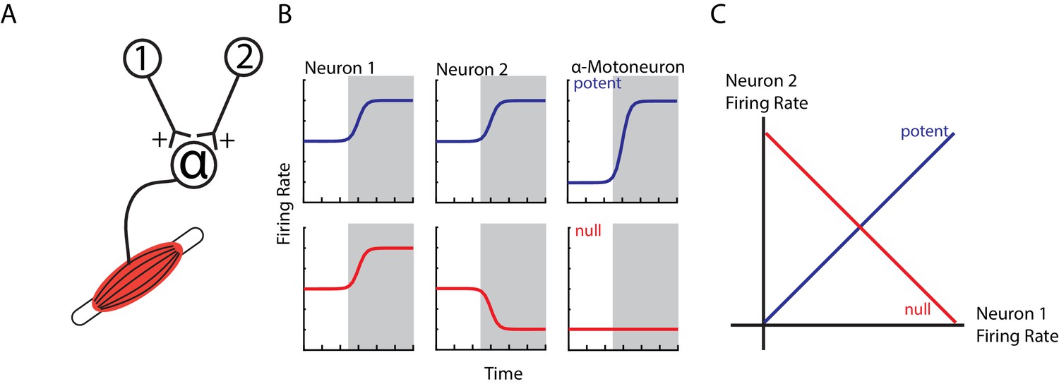
Example of orthogonal subspaces.
(A) Simple example of two neurons that synapse onto an alpha-motoneuron with equal, positive weights. (B) Top row, when both neurons increase their firing rate to an event (shaded area), their total activity is summed by the alpha-motoneuron leading to an increase in motor output (potent activity). Bottom row, when neuron one increases and neuron two decreases their firing rate, their net effect cancels at the alpha-motoneuron, thus preventing changes in motor output (null activity). (C) State space plots of the firing rates of neurons 1 and 2. Plotting the potent (blue axis) and null (red axis) activity reveals that these patterns are orthogonal with respect to each other (i.e. 90 degrees). Thus, the one-dimensional potent axis represents an orthogonal dimension to the one-dimensional null dimension.
Figure 2 with 1 supplement
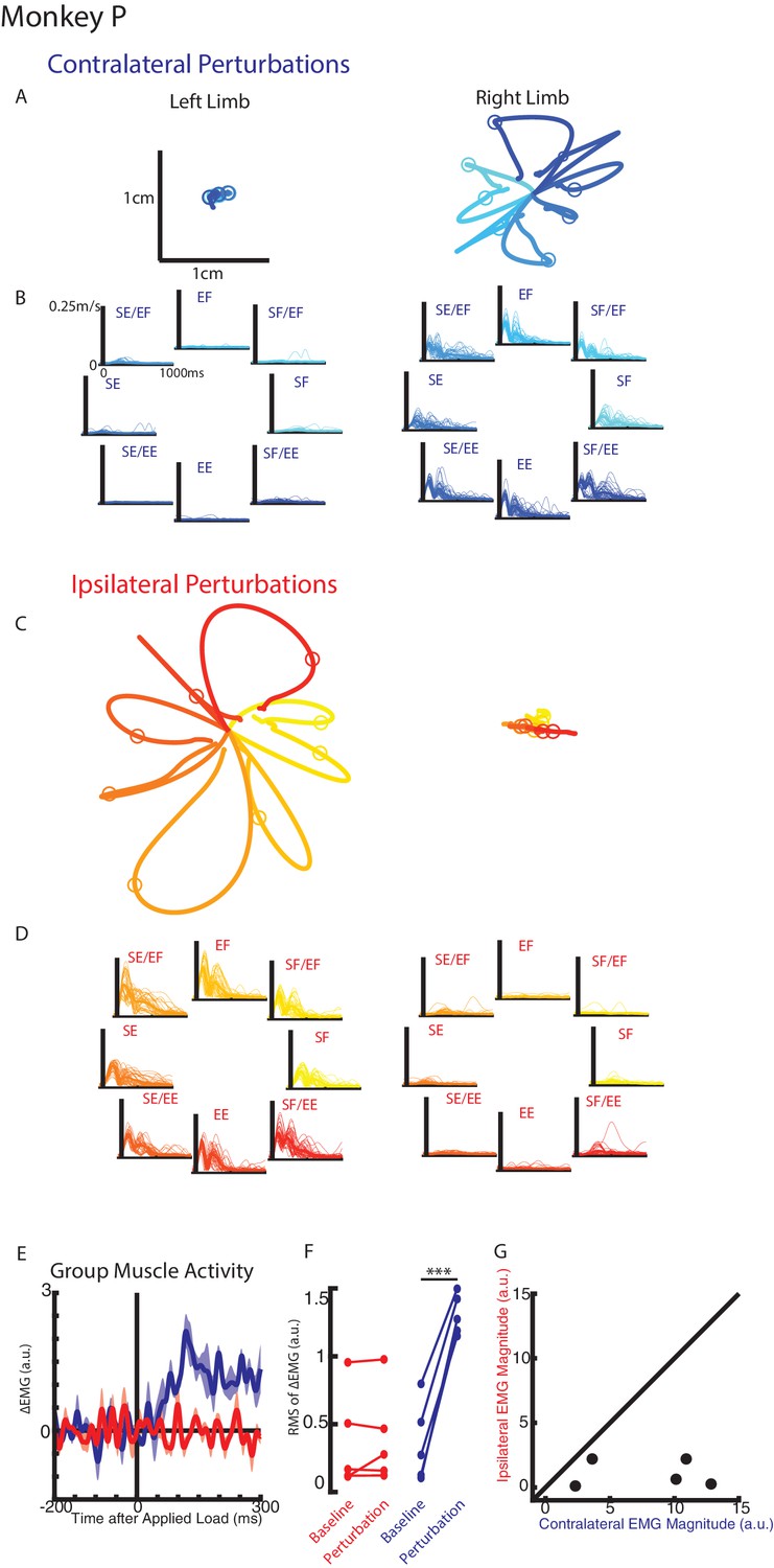
Hand kinematics when loads were applied to the contralateral or ipsilateral limbs.
(A) Average hand paths for the left and right hand from Monkey P when loads were applied to the contralateral limb (right limb). Circles indicate hand position 300 ms after the loads were applied. Left and right limb data are plotted on the same scale. (B) Single trial (thin lines) and average (thick) hand speeds when contralateral loads were applied. Black vertical line marks the onset of the load. Speed scales are the same for each load combination and for both hands. (C–D) Same as A-B for ipsilateral loads. Note, data are plotted on the same scale as in A-B. See Figure 2—figure supplement 1 showing the unperturbed hand speeds on smaller spatial and temporal scales. (E) Group average change in muscle activity recorded from the right limb of Monkey P for contralateral and ipsilateral loads. Note, for presentation purposes, EMG traces were low-pass filtered with a 3rd-order Butterworth filter with a cut-off frequency of 50 Hz. (F) Comparison of the root-mean-squared (RMS) muscle activity during the baseline and perturbation epoch. (E) Comparison of the average muscle activity for each sample in the perturbation epoch for contralateral and ipsilateral loads. ***p<0.001.
Figure 2—figure supplement 1
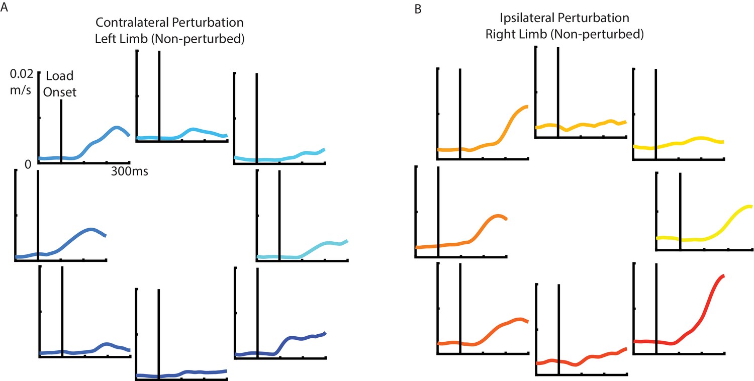
Kinematic motion of the unperturbed limb.
(A) Average hand speeds for the unperturbed (left) limb for the contralateral loads. (B) Average hand speeds for the unperturbed (right) limb for the ipsilateral loads. Black vertical line marks the onset of the load. Plotted on the same scale as A.
Figure 3 with 1 supplement

Example neuron responses for ipsilateral and contralateral loads.
(A) A neuron with significant fits for the ipsilateral (left) and contralateral loads (right). Vertical line in each panel denotes the time when the load was applied to the limb. Eight load combinations were applied to each limb and are displayed following the same format in Figure 10. Note, the firing rate scales are different between the ipsilateral and contralateral activity. Center panel shows the average firing rate in the perturbation epoch (grey regions) for each load combination. p denotes the probability values for the planar fits. (B) A neuron with a significant planar fit for contralateral loads only. (C) A neuron with a significant planar fit for ipsilateral loads only. See Figure 3—figure supplement 1 for four additional example neurons.
Figure 3—figure supplement 1

Additional example neurons.
(A–B) Example neurons with significant fits for the contralateral and ipsilateral loads. (C) Example neuron with a significant fit for contralateral loads only. (D) Example neuron with a significant fit for ipsilateral loads only.
Figure 4 with 1 supplement
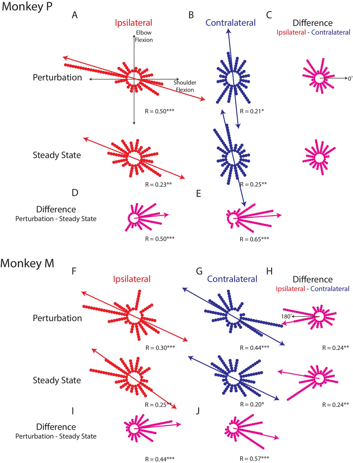
Tuning distributions in joint-torque space.
(A) Polar histograms showing the distribution of tuning curves plotted in joint-torque space for the perturbation (top) and steady-state (bottom) epoch for the ipsilateral loads. R reports the Rayleigh statistic. Red arrow shows the major axis of the bimodal distribution. Only load-sensitive neurons were included. (B) Same as A for the contralateral loads. (C) Polar histograms showing the change in tuning between the contralateral and ipsilateral loads. Neurons with no change in tuning between contralateral and ipsilateral loads would lie along the 0° axis (top). (D) Polar histogram showing the change in tuning between the perturbation and steady-state epochs for ipsilateral loads. Magenta arrows indicate major axis for the unimodal distribution. (E) Same as D for contralateral loads. (F–J) Same as A-E for Monkey M. *p<0.05, **p<0.01, ***p<0.001.
Figure 4—figure supplement 1
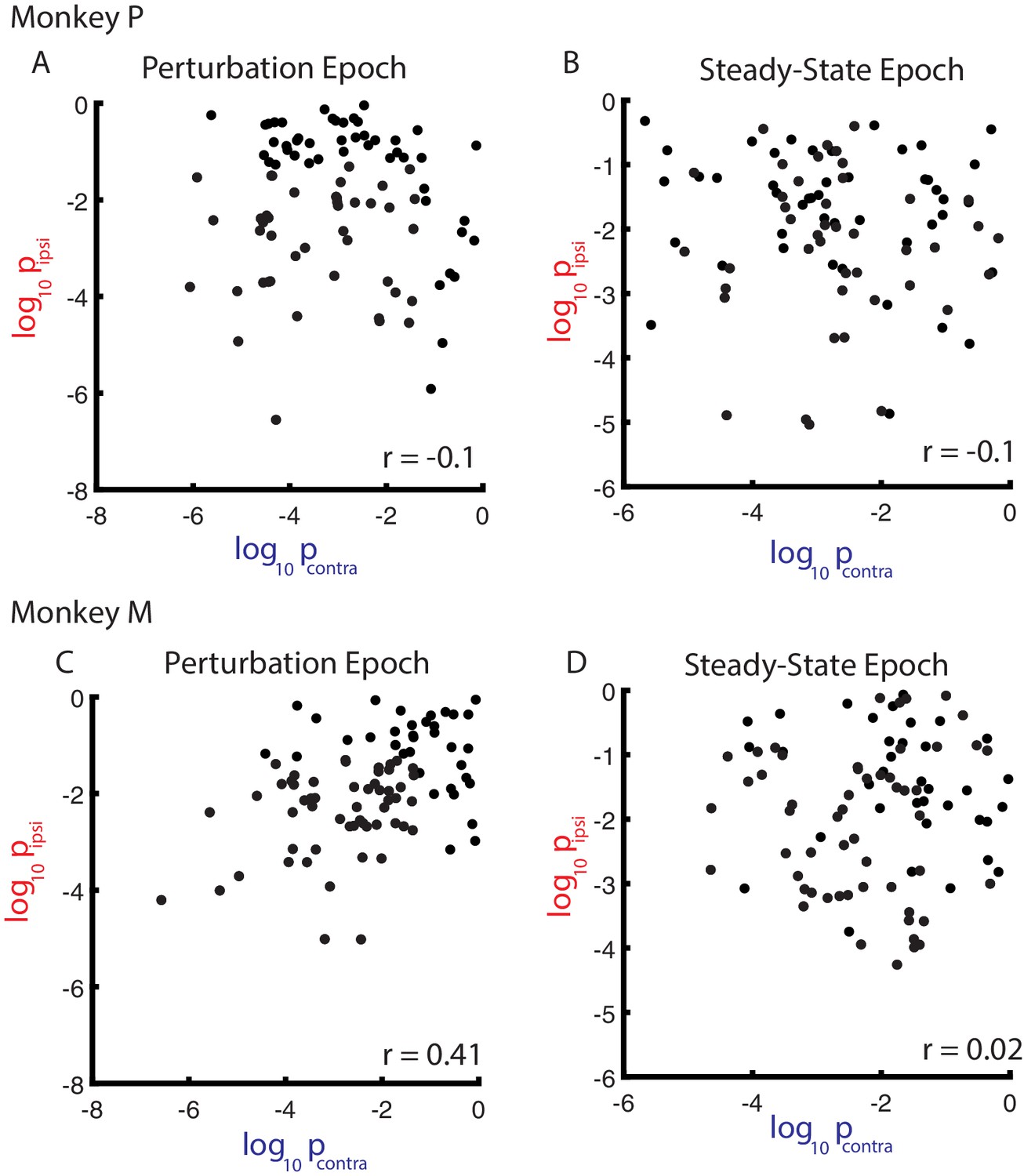
Comparison between contralateral and ipsilateral probability values.
(A) Comparison between the probability values generated from the contralateral and ipsilateral planar fits during the perturbation epoch for Monkey P. r denotes Pearson’s correlation coefficient. Note, the logarithmic axes. (B) Same as A) for the steady-state epoch. (C–D) Same as A-B) for Monkey M.
Figure 5
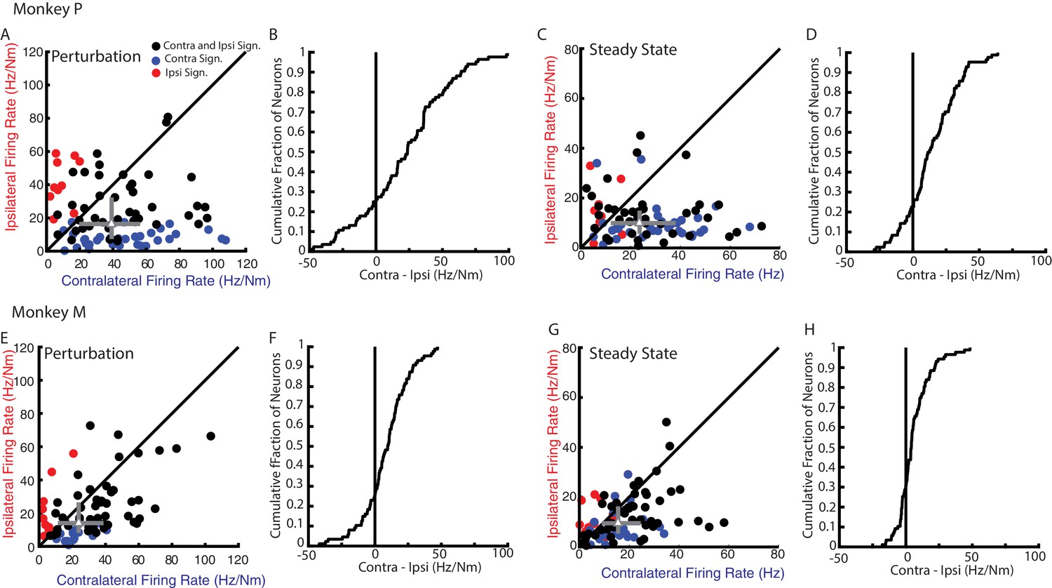
Magnitude comparison between contralateral and ipsilateral neural responses.
(A) Comparison between the contralateral and ipsilateral firing rates during the perturbation epoch for each neuron as determined by their planar fit. Black circles are neurons with significant fits for contralateral and ipsilateral loads. Blue and red circles are neurons with a significant fit for contralateral or ipsilateral loads only, respectively. Grey triangle and bars represent the median and interquartile range, respectively. (B) The cumulative distribution generated from the difference between contralateral and ipsilateral firing rates. Only neurons with a significant fit for at least one of the contexts were included. (C–D) Same as A-B for steady state. (E–H) Same as A-D for Monkey M.
Figure 6 with 1 supplement

Timing of neural responses for the contralateral and ipsilateral loads.
(A) The average change in firing rate across the population for the contralateral and ipsilateral loads. Arrows mark the onset when a significant change in baseline was detected for contralateral (blue) and ipsilateral (red) loads. Mean and SEM are plotted. All load-sensitive neurons were included. (B) Comparison of the onsets for the contralateral and ipsilateral loads. Grey triangle and bars represent the median and interquartile range, respectively. (C) The cumulative distribution generated from the difference between contralateral and ipsilateral onset times. (D) Comparison between onset differences between the contralateral and ipsilateral activity with the ratio of their activity magnitudes. r denotes Pearson’s correlation coefficient. (E–H) Same as A-D for Monkey M. (B–D, F–H) Only neurons that were load-sensitive and had significant onsets for both contexts were included.
Figure 6—figure supplement 1

Onset timing while controlling for magnitude effects.
We analyzed a subset of neurons with an absolute magnitude difference between the contralateral and ipsilateral activity that was <20 Hz. (A) Cumulative distribution of the magnitude difference. (B) Comparison between contralateral and ipsilateral timing. Grey triangle denotes the median and grey bars denote the interquartile range. (C) Cumulative distribution of the onset differences between contralateral and ipsilateral loads. (D–F) Same as A-C for Monkey M.
Figure 7
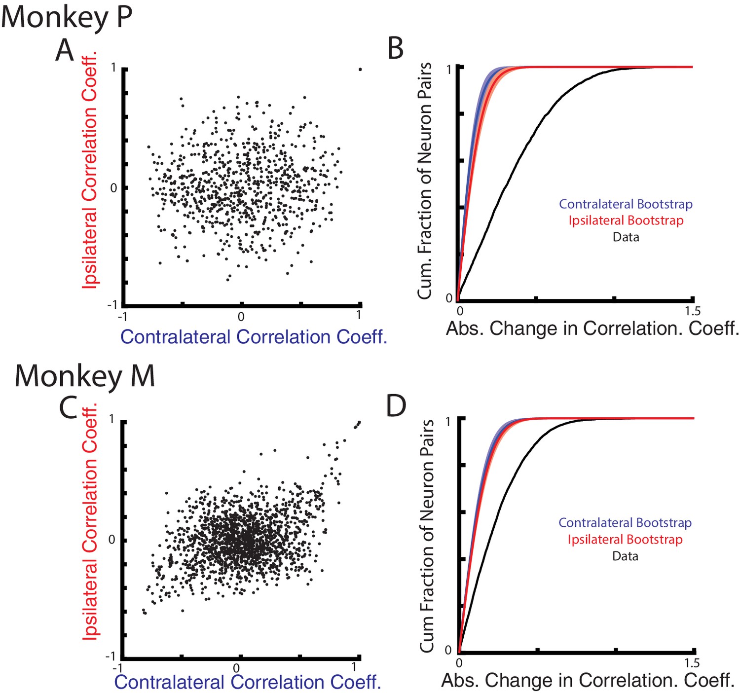
Correlation changes between neurons for ipsilateral and contralateral loads.
(A) Comparison of the pairwise correlation coefficients between neurons during the ipsilateral and contralateral loads. (B) The cumulative sum of the absolute change in the pairwise correlation coefficient between the ipsilateral and contralateral loads (black). A bootstrap distribution was generated by separating ipsilateral trials into two distinct groups and calculating the absolute change in pairwise correlation coefficient (red trace). This was repeated 1000x. Shaded region shows three standard deviations from the mean. This was repeated for the contralateral data (blue). (C–D) Same as A-B for Monkey M.
Figure 8
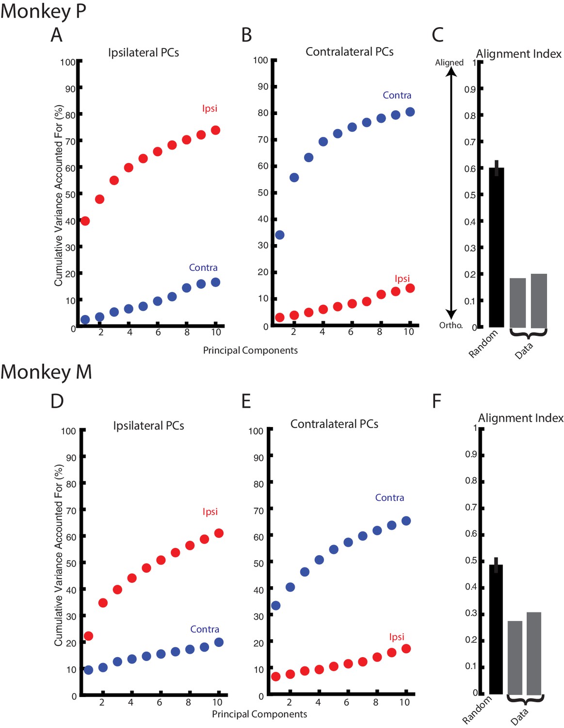
Ipsilateral and contralateral activity reside in nearly orthogonal subspaces.
(A) The cumulative variance explained of the ipsilateral and contralateral activity from the ten largest ipsilateral principle components. (B) The cumulative variance explained of the ipsilateral and contralateral activity from the ten largest contralateral principle components. (C) The alignment index generated by randomly sampling from the data covariance matrix (black, mean + standard deviation) and the two indices generated from the ipsilateral and contralateral principle components (grey). (D–F) Same as A-C for Monkey M.
Figure 9
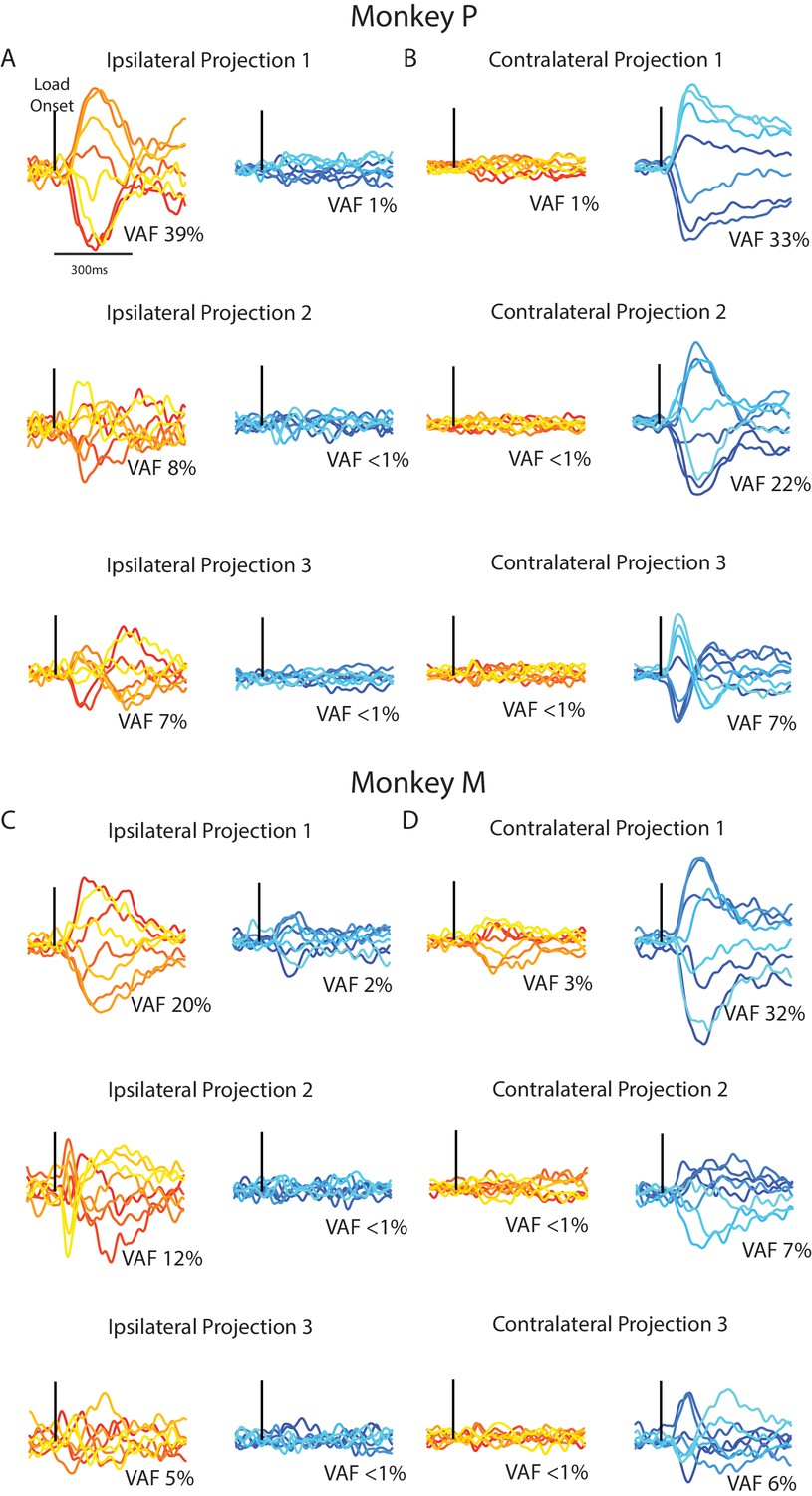
Time series from the ipsilateral and contralateral dimensions.
(A) For Monkey P, the time series generated by projecting the ipsilateral (left) and contralateral (right) activity onto the three ipsilateral. Black line indicates when the load was applied. (B) Same as A for the three contralateral dimensions. (C–D) Same A-B for Monkey M.
Figure 10
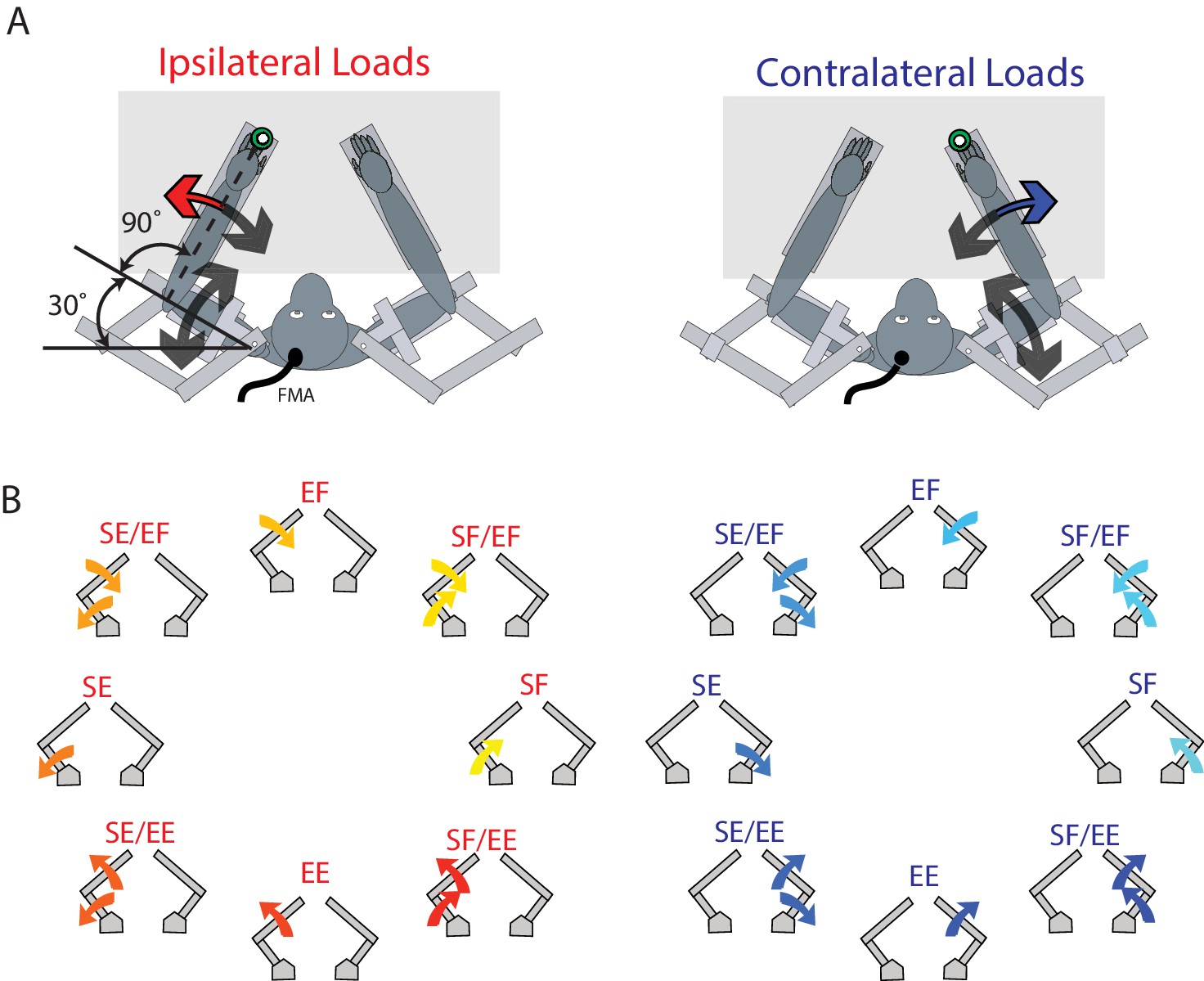
Experimental set-up.
(A) The monkey’s left and right arms were supported by the exoskeleton. Monkeys were trained to return their hand to the goal target (green) when mechanical loads were applied to the left (ipsilateral; red arrow) and right (contralateral; blue arrow) hand. Visual feedback of their hand was presented as a white cursor. The target was placed such that to reach the target monkeys required to flex their shoulder 30° and place their elbow at 90°. (B) For ipsilateral and contralateral loads, combinations of flexion and extensions torques were applied to the shoulder and elbow joints. Arrows show the net applied torque for each load combination. Abbreviations: SF shoulder flexion, SE shoulder extension, EF elbow flexion, EE elbow extension, FMA floating micro-electrode array.
Additional files
-
Supplementary file 1
Comparison of Rayleigh statistic between the non-overlapping subset of neurons and the original neuron population.
Significance assessed based on sampling from a uniform distribution. *p<0.05, **p<0.01, ***p<0.001
- https://doi.org/10.7554/eLife.48190.016
-
Supplementary file 2
Comparison of firing magnitude between the non-overlapping subset of neurons and the original neuron population.
- https://doi.org/10.7554/eLife.48190.017
-
Supplementary file 3
Comparison of onset timing between the non-overlapping subset of neurons and the original neuron population.
- https://doi.org/10.7554/eLife.48190.018
-
Transparent reporting form
- https://doi.org/10.7554/eLife.48190.019
Download links
A two-part list of links to download the article, or parts of the article, in various formats.
Downloads (link to download the article as PDF)
Open citations (links to open the citations from this article in various online reference manager services)
Cite this article (links to download the citations from this article in formats compatible with various reference manager tools)
Independent representations of ipsilateral and contralateral limbs in primary motor cortex
eLife 8:e48190.
https://doi.org/10.7554/eLife.48190


