Structure of the two-component S-layer of the archaeon Sulfolobus acidocaldarius
- Living Systems Institute, University of Exeter, United Kingdom
- Faculty of Environment, Science and Economy, University of Exeter, United Kingdom
- Faculty of Health and Life Sciences, University of Exeter, United Kingdom
- Department of Theoretical Biophysics, Max Planck Institute for Biophysics, Germany
- Malopolska Centre of Biotechnology, Jagiellonian University, Poland
- Institute of Psychiatry and Neurosciences of Paris, Inserm UMR1266 - Université Paris Cité, France
- GHU Psychiatrie et Neurosciences de Paris, France
- Henry Wellcome Building for Biocatalysis, Biosciences, Faculty of Health and Life Sciences, University of Exeter, United Kingdom
Figures
Figure 1 with 6 supplements

Atomic model of S. acidocaldarius S-layer protein SlaA at pH 4.
(a, b), SlaA30–1069 atomic model obtained by single-particle cryo electron microscopy (cryoEM) in ribbon representation and cyan–grey–maroon colours (N-terminus, cyan; C-terminus, maroon) with α-helices highlighted in orange. (c, d) SlaA atomic models highlighting six domains: D130–234 (orange), D2235–660,701–746 (purple), D3661–700,747–914 (cyan), D4915–1074 (yellow), D51075–1273 (pink), and D61274–1424 (grey). D5 and D6 were predicted using Alphafold. A flexible hinge exists between D4 and D5. D5 and D6 are thus free to move relative to D1–D4 in the isolated SlaA particle (represented by a curved grey arrow between a stretched (c) and a flapped (d) conformation). Scale bar, 20 Å.
Figure 1—figure supplement 1

Relion processing workflow for the pH 4 dataset of SlaA.
Figure 1—figure supplement 2

Representative cryoEM micrographs and 2D classes for SlaA.
Representative cryoEM micrographs (from a total of 3687 for (a), 3163 for (b), and 5046 for (c)). (d–f) 2D classification examples of S. acidocaldarius polished SlaA particles at pH 4 (a, d), pH 7 (b, e), and pH 10 (c, f). Scale bars (a–c) 100 nm; (d–f) 50 Å.
Figure 1—figure supplement 3
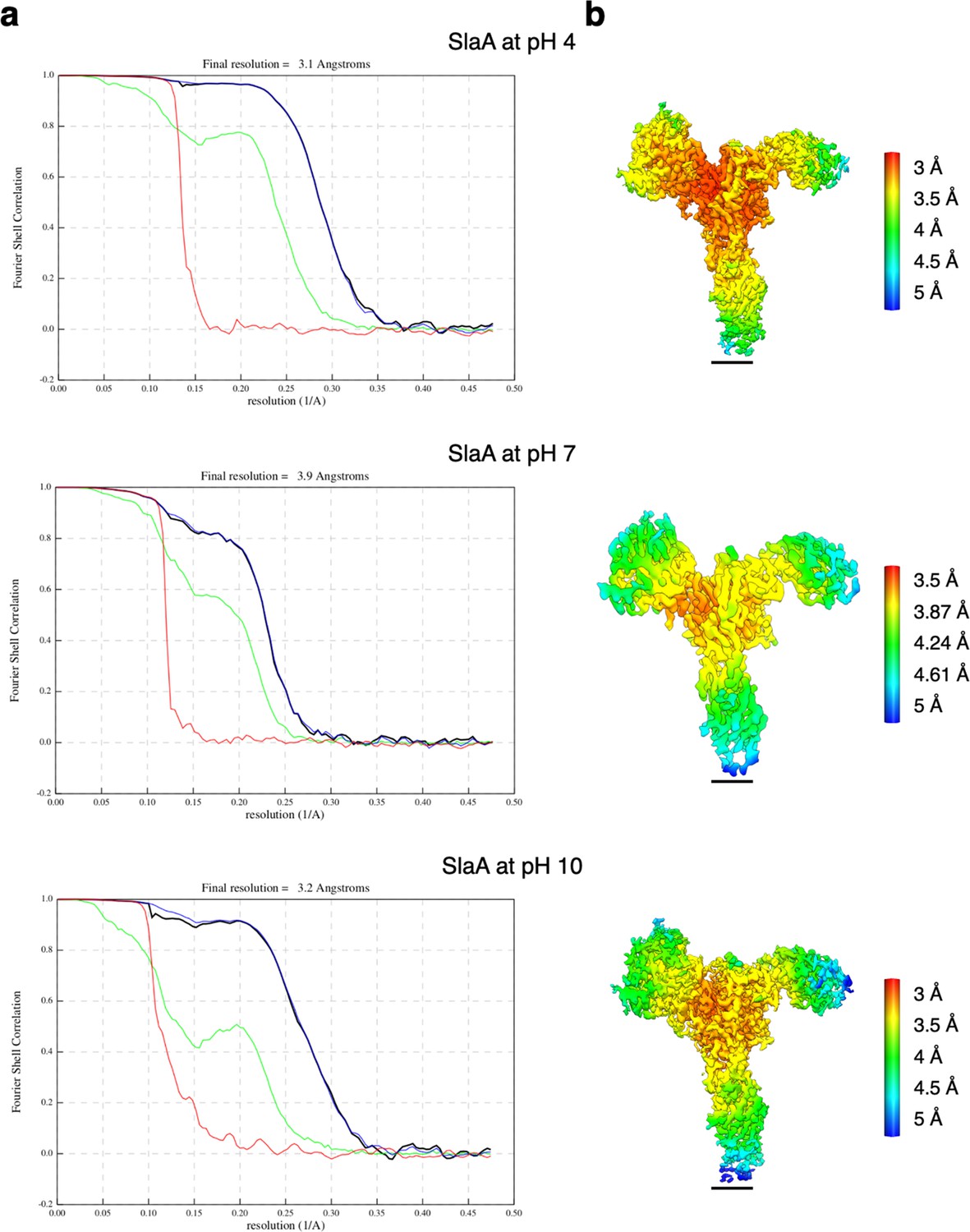
Resolution estimation for the cryoEM maps of SlaA.
(a) Gold-standard Fourier Shell Correlation (FSC) and (b) local resolution estimations for the SlaA map obtained at pH 4, 7, and 10. Red, phase randomised masked; green, unmasked; blue, masked; black, corrected. Scale bar, 20 Å.
Figure 1—figure supplement 4
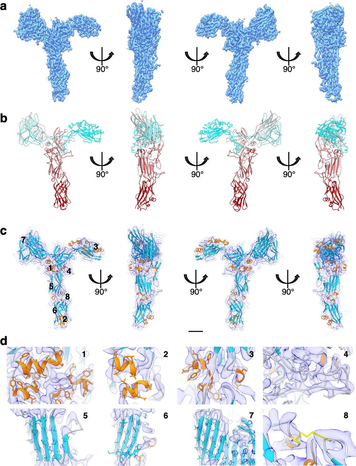
SlaA30–1069 cryo electron microscopy (cryoEM) map and atomic model.
(a) CryoEM map of SlaA30–1069 at 3.1 Å global resolution. (b) Atomic model of SlaA30–1069 (ribbon representation, cyan–grey–maroon colours; N-terminus, cyan; C-terminus, maroon). (c) Fitting of the atomic model (ribbon representation) into the cryoEM map (transparent purple). The loop regions are in grey, α-helices in orange, β-sheets in turquoise, and the disulphide bridge in yellow. (d) Close-ups of three example regions of β-sheets, α-helices, and the disulphide bridge. Locations of the close-ups are labelled in (d) as 1-8 in (c). Scale bar in (a–c) 20 Å.
Figure 1—figure supplement 5
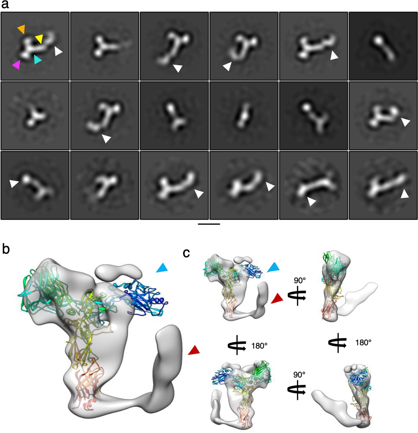
SlaA flexibility.
(a) 2D classification of negatively stained micrographs of SlaA purified from S. acidocldarius. The white arrowheads point at domains D5 and D6 in different orientations, highlighting the flexibilit of these domains relative to the rest of the protein (D1-4). The arrowheads in the first class highlight D1 (orange), D2 (purple), D3 (cyan), and D4 (yellow). Scale bar, 100 Å. (b) Low-resolution 3D refinement of Saccharolobus solfataricus SlaA (transparent grey; 13.5 Å resolution) superimposed with the atomic model of S. acidocaldarius SlaA (rainbow ribbon). While in the S. solfataricus map, the N-terminus (blue arrowhead) is not resolved (due to flexibility), the C-terminus is visible (red arrowhead) and in a ‘closed’ conformation, reminiscent of the Alphafold predications shown in Figures 1—3, as well as Figure 1—figure supplement 6. (c) Map and model from (b) shown in different orientations.
Figure 1—figure supplement 6

Five Alphafold predictions of SlaA914–1424.
(a–e) SlaA30–1069 is shown in ribbon representation and cornflower blue; glycans are in ball-stick representation and rusty brown. The Alphafold predictions are coloured according to domains, highlighting domains D5 (pink) and D6 (grey). Residues 914–1069 (D4 in yellow) at the C-terminus of SlaA30–1069 were included in the prediction to aid alignment between SlaA30–1069 and D5–D6. The predicted D4 largely overlaps with the cryoEM structure of the SlaA30–1069 N-terminus. The black arrowhead (a) indicates the intramolecular hinge loop. (f) pLDDT (per-residue confidence score) plot showing the per-residue confidence metric of the predicted models. The dashed line marks the threshold of predicted LDDT = 70, above which the structures are expected to be modelled with high confidence. Scale bar, 20 Å.
Figure 2 with 1 supplement

N-glycosylation of S.acidocaldarius SlaA.
(a) Atomic model of SlaA in ribbon representation. SlaA30–1069 as solved by cryoEM is in cornflower blue; SlaA1070–1424 as predicted by Alphafold is in purple (boxed). 19 Asn-bound N-glycans were modelled into the cryoEM map of in SlaA30–1069 (glycans rusty brown sticks, Asn in orange). In the glycans, O atoms are shown in red, N in blue, and S in yellow. The inset shows the Alphafold model of SlaA1070–1424 (D5 and D6), where eight likely glycosylated Asn residues (Peyfoon et al., 2010) are highlighted as orange sticks. Scale bar, 20 Å. (b–d) Example close-ups of glycosylation sites with superimposed cryoEM map (blue mesh). (b) Shows the full hexasaccharide on Asn377, (c) shows GlcNAc2 on Asn559, and (d) shows a pentasaccharide lacking Glc1 on Asn714. (e) List of glycosylation sites and associated glycans of SlaA30–1069. The schematic glycan representation (f) is equivalent to (Peyfoon et al., 2010). Blue square, N-acetylglucosamine; green circle, mannose; pink circle, 6-sulfoquinovose; blue circle, glucose. (g, h) GlycoSHIELD models (red, orange) showing the glycan coverage of the protein (solid grey). Glycan shields corresponding to glycosylation sites visualised by cryoEM are coloured red, glycan shields with the Alphafold model of the SlaA C-terminus are shown in orange.
Figure 2—figure supplement 1
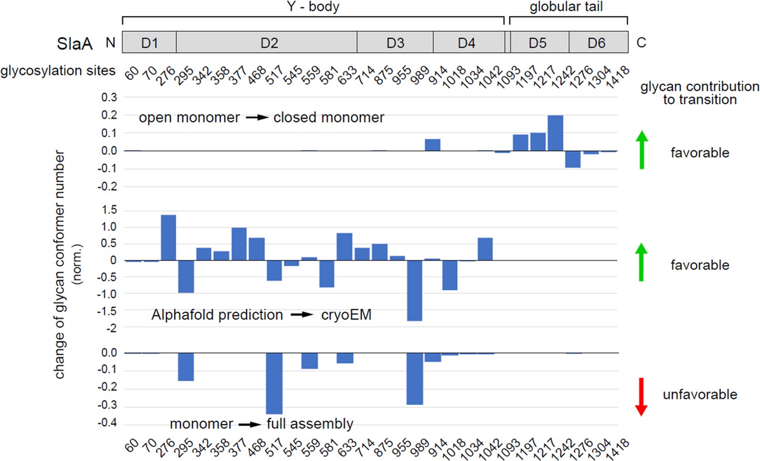
Entropic contribution of glycans to protein conformation.
Position of N-glycosylated sites and globular domains on SlaA primary structure (upper panel) and changes of the number of possible N-glycan conformers at each glycosylated site (bar graphs). Top, SlaA with stretched (open) vs. flapped D5–D6 domains (closed). Middle, SlaA Y-body predicted by Alphafold v2.2.0 vs. experimental cryo electron microscopy (cryoEM). Bottom, monomer in isolation vs. in the assembled structure. Bar charts show changes of glycan conformer numbers at individual glycosylation sites normalised by global changes for all glycans. Positive and negative values indicate an increase or a decrease of possible glycan conformations, respectively, indicative of favourable and unfavourable entropic contributions. The seven last N-glycans of the protein were not taken into account for the Alphafold–cryoEM comparison plot, changing the scale of the Y axis compared to the two other plots. Green and red arrows on the right side of the figure indicate a total increase or decrease of glycan conformers during the transition between the two conformations of the protein that were compared in each plot, indicative of favourable and unfavourable entropic contributions to the conformation transition.
Figure 3 with 3 supplements

Structural comparison and electrostatic surface potentials of S.acidocaldarius SlaA at different pH conditions.
(a) SlaA30–1069 cryo electron microscopy (cryoEM) maps at pH 4 (light blue, res. 3.1 Å), pH 7 (orange, res. 3.9 Å), and pH 10 (magenta, res. 3.2 Å). (b) r.m.s.d. (root-mean-square deviation) alignment between SlaA30–1069 atomic models at pH 4 and 10. Smaller deviations are shown in blue and larger deviations in red, with mean r.m.s.d. = 0.79 Å. Electrostatic surface potentials of SlaA at pH 4 (c), pH 7 (d), and pH 10 (e). Models include Alphafold-predicted C-terminal domains (in closed conformation). Surfaces are coloured in red and blue for negatively and positively charged residues, respectively. White areas represent neutral residues. In (c), some areas occupied by glycans are circled; the arrow points at one of the 6-sulfoquinovose residues displaying a negative charge at pH 4. Scale bar, 20 Å.
Figure 3—figure supplement 1
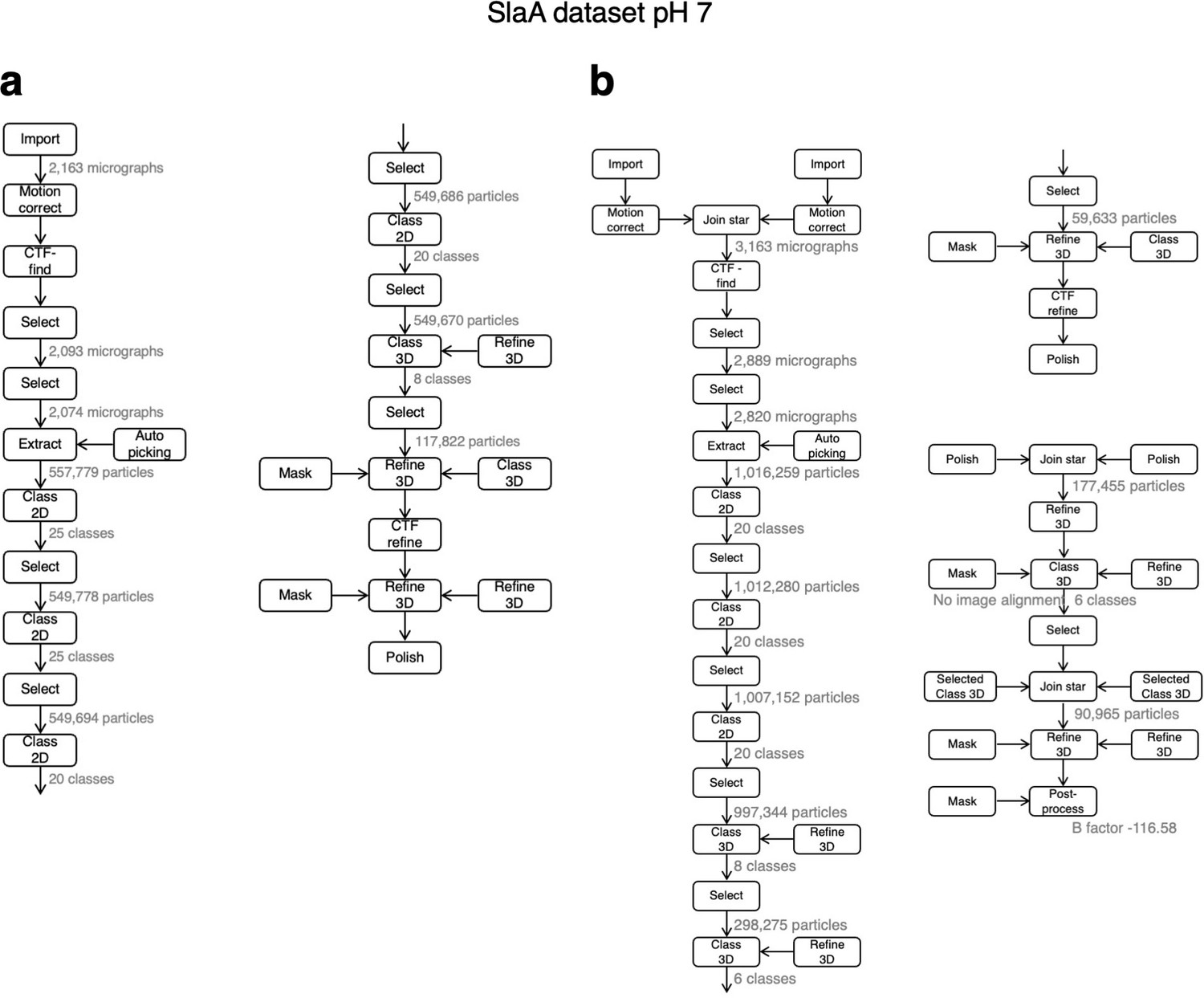
Relion processing workflow for pH 7 dataset.
The image processing pipeline incuded the collection of two datasets (a and b), which were subsequently merged.
Figure 3—figure supplement 2
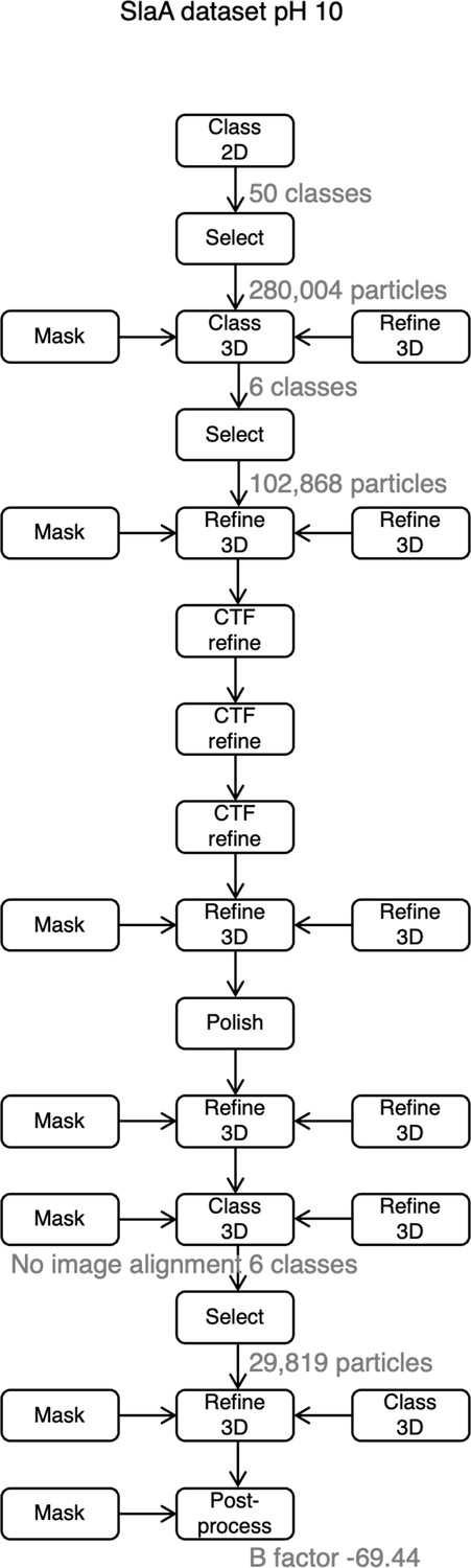
Relion processing workflow for pH 10 dataset.
Figure 3—figure supplement 3
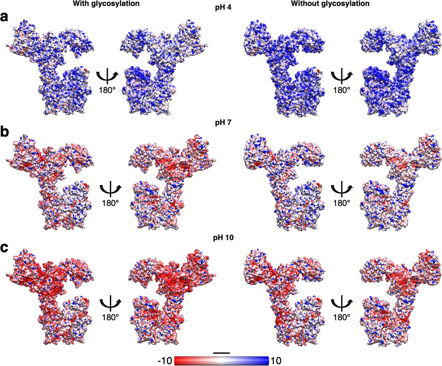
Impact of glycosylation on the electrostatic surface charge of SlaA at different pH values.
Comparison of the SlaA electrostatic surface charge with (left) and without (right) glycans at pH 4 (a), 7 (b), and 10 (c). The glycosylation increases the overall surface negative charge of SlaA, particularly noticeable at pH 7 and 10. Scale bar, 20 Å.
Figure 4 with 4 supplements

S. acidocaldarius SlaA assembly into exosome-bound S-layers.
(a) Extracellular view of assembled SlaA monomers in rainbow colours and surface representation. (b) Extracellular view of assembled SlaA in ribbon representation with SlaA dimers forming a hexagonal pore highlighted in shades of red and yellow. Each dimer spans two adjacent hexagonal pores. (c) Side view of the SlaA lattice (blue, N-terminus; red, C-terminus). It is possible to distinguish an outer zone (OZ) formed by domain D1, D2, D3, and D4, and an inner zone (IZ) formed by domains D5 and D6. (d) One SlaA monomer (surface representation, N-terminus cyan, grey, C-terminus maroon) is highlighted within the assembled array. The long axis of each SlaA monomer (dashed line) is inclined by a 28° relative to the curved surface of the array (solid line). (e) The location of each SlaA domain within the S-layer. (f–h) SlaA glycans modelled with GlycoSHIELD in the assembled S-layer. (f) Shows the extracellular view; (g) shows the intracellular view; (h) shows insets of (f) at higher magnification without (left) and with (right) glycans. Glycans fill gaps unoccupied by the protein and significantly protrude into the lumen of the triangular and hexagonal pores. Scale bars in (a–d, f–h) 10 nm; in (e) 20 Å.
Figure 4—figure supplement 1

Subtomogram averaging of the S-layer on exosomes and fitting of SlaA.
CryoEM map of the S-layer assembled on exosomes in extracellular (a), intracellular (b), and side (c) views at 11.2 Å resolution. The membrane-distal face of the map is shown in magenta, and the membrane proximal face is shown in cyan. (d–f) Fitting of the SlaA hexamer model into the S-layer map. SlaA is shown in ribbon representation in different colours, the map is depicted in transparent grey. (g–i) Fitting of six SlaA monomers around a triangular pore. Scale bar, 10 nm.
Figure 4—figure supplement 2
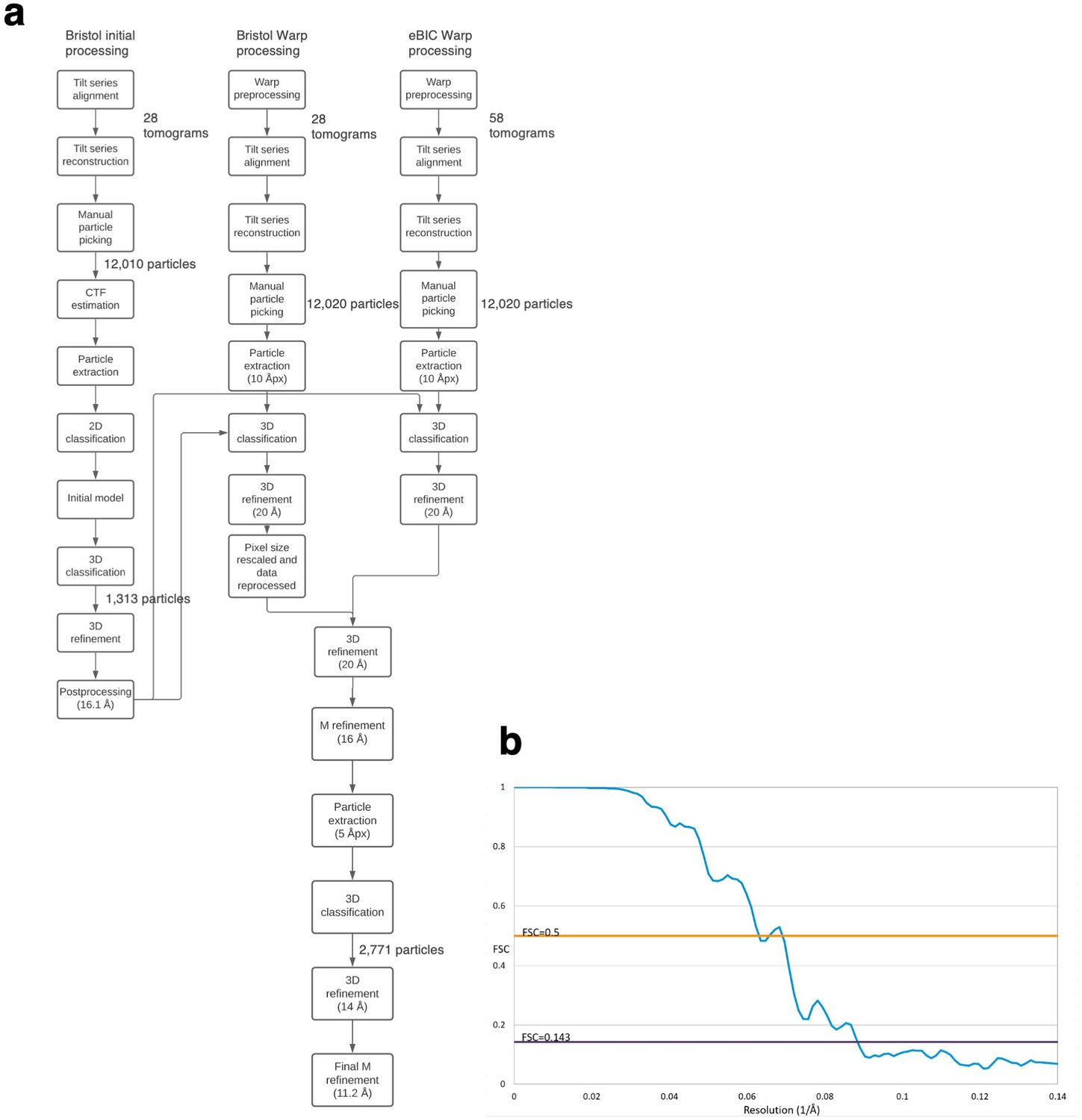
CryoET processing, STA and resolution estimation.
(a) CryoET and STA workflow using Warp–Relion–M. (b) Gold-standard FSC of the STA map.
Figure 4—figure supplement 3
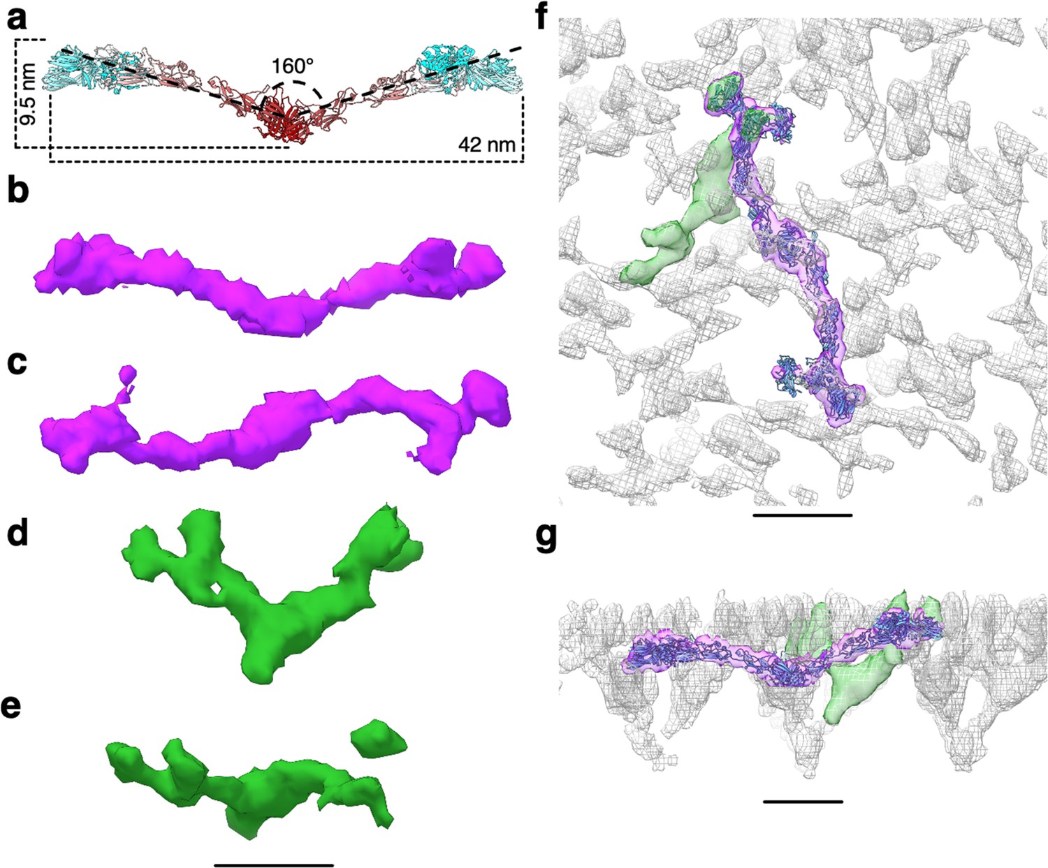
Comparison between current and previously reported (Gambelli et al., 2019) S. acidocaldarius SlaA assembly models.
(a) Side view of the SlaA dimer (ribbon representation; cyan, N-terminus; maroon, C-terminus). Within the dimer, the long axes of two SlaA monomers include an angle of ~160°. The dimer has a height of 9.5 nm and a length of 42 nm. (b–e) CryoEM densities extrapolated from the S-layer map published in 2019 (Gambelli et al., 2019). The purple density in (b) and (c) (side and extracellular views, respectively) contains the SlaA dimer as presented in this work (f, g). The green density in (d) and (e) (side and extracellular views, respectively), represents the SlaA dimer as reported previously (Gambelli et al., 2019). (f, g) show the atomic model of the SlaA dimer in (a) and the cryoEM densities in (b–e) fitting the S-layer cryoEM map (grey mesh) presented in Gambelli et al., 2019. Scale bar, 10 nm.
Figure 4—figure supplement 4
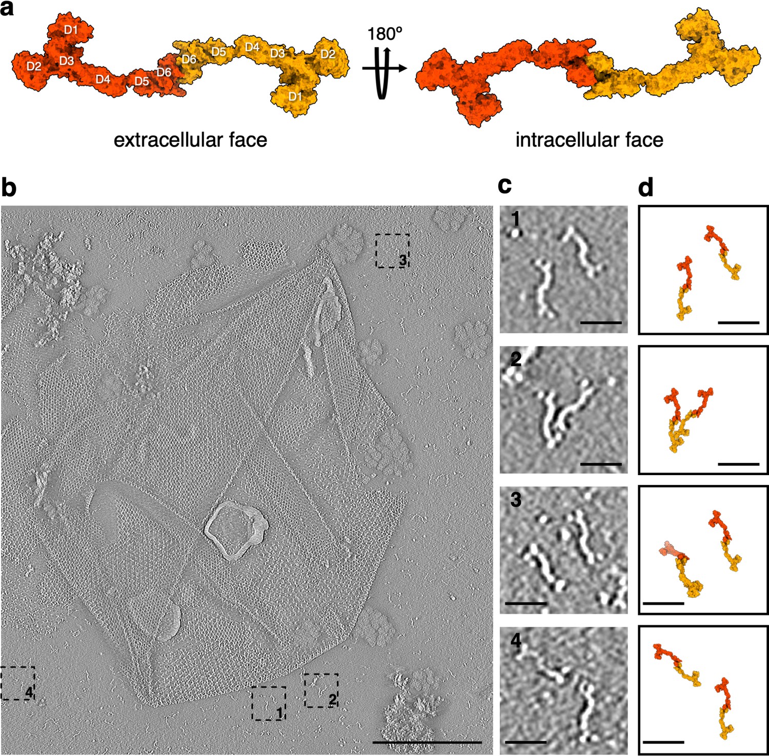
Isolated SlaA-only S-layer from S.acidocaldarius.
(a) Surface representation of the atomic model of the SlaA dimer, as it occurs in the S-layer. (b) Negative stain electron tomography of isolated SlaA-only S-layer. (c) 1–4 are cut-outs from (b) showing dimeric SlaA with their respective positions marked in (b). (d) Atomic models from (a) scaled and superimposed with the dimers seen in negative stain tomography (c). Scale bar, (b) 200 nm; scale bars, (c, d) 25 nm.
Figure 5 with 6 supplements

S. acidocaldarius S-layer assembly.
(a, b) SlaB trimer (ribbon representation, N-terminus, cyan; C-terminus, maroon) as predicted by Alphafold v2.2.0 (Jumper et al., 2021). (c–e) Ribbon representation of the assembled SlaA and SlaB components of the S-layer. (c), (d), and (e) show the external face, the pseudo-periplasmic face, and a side view, respectively. SlaA proteins around each hexagonal pore are shown in different colours. SlaB trimers are shown in shades of yellow and orange (N-termini are red-orange shades and C-termini are yellow). Scale bar, (a, b) 20 Å; (c–e) 10 nm.
Figure 5—figure supplement 1
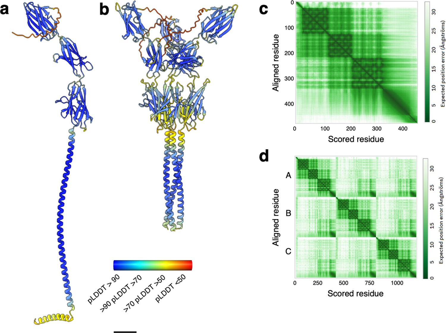
Alphafold v2.2.0 predictions of SlaB monomer and trimer.
(a, b) Alphafold v2.2.0 predictions of SlaB monomer and trimer, respectively. The ribbon is coloured by pLDDT (per-residue confidence score) where red indicates low, and blue high confidence. The trimeric coiled coil of the SlaB trimer (b) is truncated at residue 400, and the complete trimeric coiled coil (Figure 5d) was predicted using SymmDock. (c, d) PAE (predicted aligned error) plots for (a) and (b), respectively. Scale bar, 20 Å.
Figure 5—figure supplement 2

Structural prediction of S. acidocaldarius SlaB.
(a) Structure of SlaB as predicted by Alphafold v2.2.0 (ribbon representation, cyan–grey–maroon from N-terminus to C-terminus). Amino acids from 1 to 24 (blue) are predicted as signal peptide by InterPro. Amino acids from 448 to 470 (yellow) are predicted as transmembrane helix by TMHMM-2.0. (b) Putative N-glycosylation sites are labelled as predicted by GlycoPP v1.0. (c) SlaB sequence with predicted N-glycosylated residues in green. (d) Table showing predicted N-glycosylation distribution across four SlaB domains. SlaB trimer (as predicted by Alphafold v2.2.0) surface representation showing hydrophobicity (from most hydrophilic in dark cyan to most hydrophobic in gold) in (e), and electrostatic surface potential (from mostly negative in red, to mostly positive in blue) in (f). The arrow in (e) highlights the predicted hydrophobic transmembrane region. (f) Negatively charged patches (red) in the N-tremini of SlaB may electrostatically interact with the mostly positively charged SlaA. Scale bar, 20 Å.
Figure 5—figure supplement 3
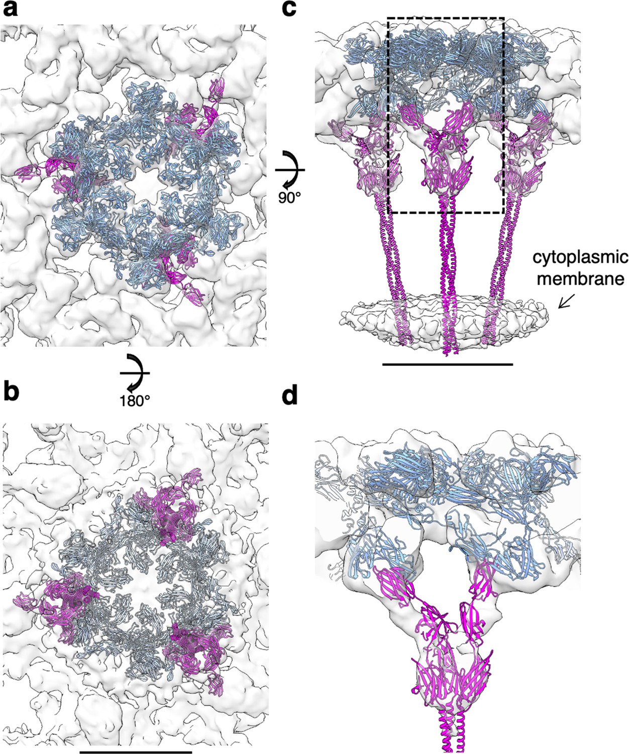
Subtomogram average of the exosome-bound S-layer and SlaB fitting.
(a–d) SlaA hexamer (cornflower blue) and SlaB trimer (magenta) fitting into the cryoEM map. (d) Cross-section through the boxed region in (c), showing the interaction between SlaA and SlaB. Scale bar, 10 nm.
Figure 5—figure supplement 4
Structure of archaeal and bacterial S-layer proteins.
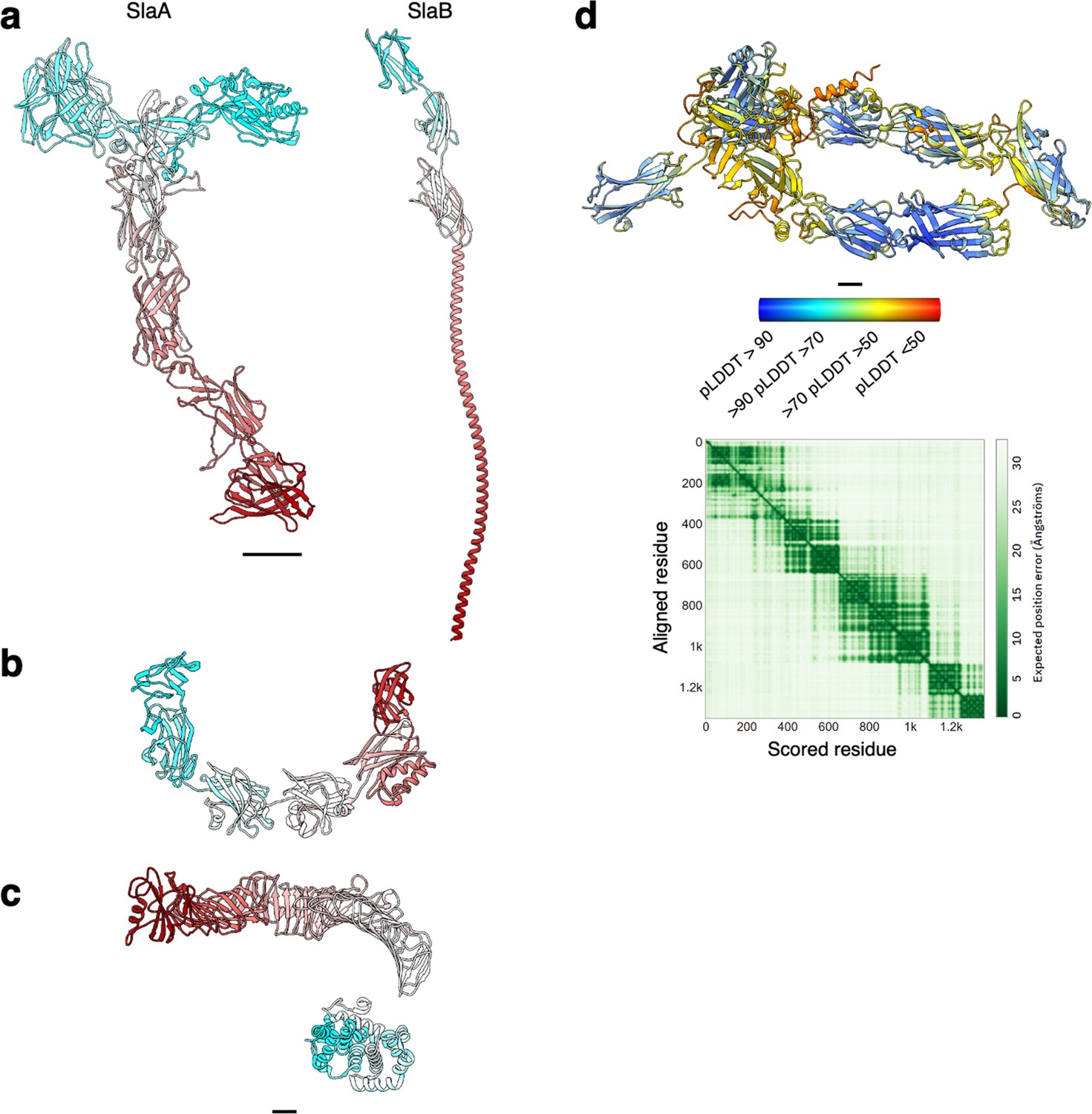
(a–c) Atomic models are shown in ribbon representation in cyan–grey–maroon from the N-terminus to the C-terminus. S. acidocaldarius SlaA (domains D5 and D6 as predicted by Alphafold v 2.2.0) and SlaB (as predicted by Alphafold v.2.2.0) are in (a), H. volcanii csg (PDB ID: 7PTR, http://dx.doi.org/10.2210/pdb7ptr/pdb) is shown in (b), and C. crescentus RsaA (N-terminus PDB ID: 6T72, http://dx.doi.org/10.2210/pdb6t72/pdb, C-terminus PDB ID: 5N8P, http://dx.doi.org/10.2210/pdb5n8p/pdb) is depicted in (c). (d) Atomic model of SlaA from M. sedula (UNIPROT A4YHQ8, as predicted by Alphafold v2.2.0) and PAE (predicted aligned error) plot. The model is shown in ribbon representation coloured by pLDDT (per-residue confidence score) where red indicates very low confidence and blue very high. Scale bar, 20 Å.
Figure 5—figure supplement 5

Stability and charge heatmaps for S. acidocaldarius SlaA30–1069, SlaA, and SlaB.
(a, c, e) Calculated folded state stability heatmaps for SlaA30–1069 (a), SlaA (c), and SlaB (e), respectively. SlaA30–1069, SlaA, and SlaB predicted to be stable across pH 2–8. (b, d, f) calculated charged heatmaps for SlaA30–1069 (b), SlaA (d), and SlaB (f), respectively. Surface charge shifts from positive to negative for SlaA30–1069 and SlaA from pH 2 to 8, whereas SlaB shows a largely consistent positive charge.
Figure 5—figure supplement 6
Stability and charge heatmaps for C.crescentus and H. volcanii S-layer proteins.
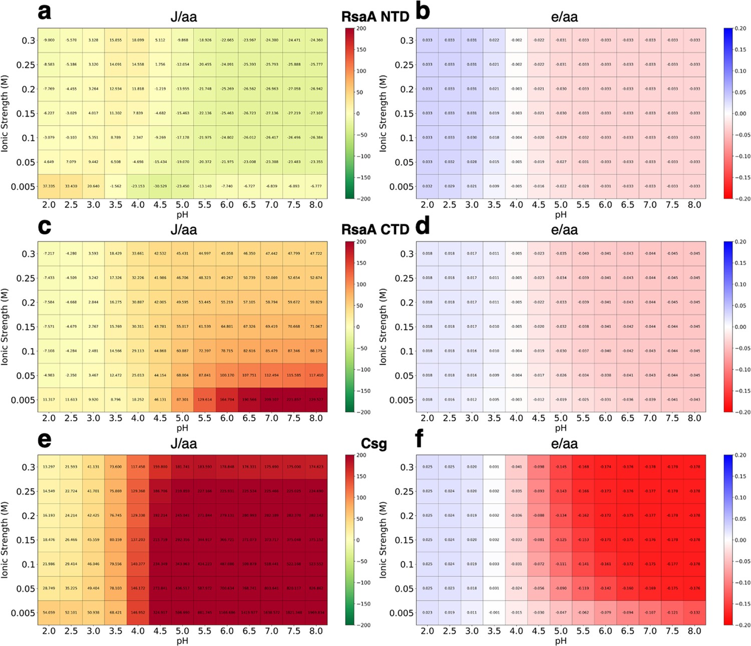
(a, c, e) calculated folded state stability heatmaps for C. crescentus S-layer protein RsaA N-terminus (a) and C-terminus (c) domains, and H. volcanii S-layer protein csg (e). The RsaA N-terminus domain is predicted to be largely stable across pH 2–8; the RsaA C-terminus domain is predicted to become unstable at elevated pH and low ionic strength; csg’s stability is aparently greatly affected at neutral and high pH. (b, d, f) calculated charged heatmaps for RsaA N-terminus (b) and C-terminus (d) domains, and csg (f). RsaA’s and csg’s surface charge shifts from positive to negative from pH 2 to 8. Csg shows a dramatic difference in surface charge from pH 3 to 5, becoming negatively charged.
Videos
Video 1
Atomic structure and glycosylation of SlaA30–1069. The SlaA30–1069 cryo electron microscopy (cryoEM) map is shown in cornflower blue.
The atomic structure is shown in ribbon representation and coloured in cyan–grey–maroon. N-terminus, cyan; C-terminus, maroon. The glycosylated Asn residues are in orange and the glycans are represented as balls and sticks. C, medium blue; N, dark blue; O, red; S, yellow.
Video 2
Flexibility of SlaA.
Sequence of 2D classifications of negatively stained SlaA obtained in Relion 3. D2-4 were aligned, showing the flexibility of D1, D5, and D6.
Video 3
Comparison of SlaA30–1069 structure at pH 4 and 10. Root-mean-square deviation (r.m.s.d.) alignment between SlaA30–1069 atomic models at pH 4 and 10.
Smaller deviations are shown in blue and larger deviations in red, with mean r.m.s.d. = 0.79 Å, as in Figure 3b.
Video 4
Model of the assembled S. acidocaldarius S-layer.
Additional files
-
Supplementary file 1
CryoEM statistics.
(a) Statistics of data collection, 3D reconstruction, and validation. (b) Mapping of glycan residues from the structure file to residues of the GLYCAM force field or the newly charge-derived SG0 and SG4 residues, representing the 1-substituted and 1,4-substituted SMA. (c) RESP charges derived for residue SG0 on the HF/6-31G*//HF/6-31G* level of theory (see Methods for details). (d) RESP charges derived for residue SG4 on the HF/6-31G*//HF/6-31G* level of theory (see Methods for details).
- https://cdn.elifesciences.org/articles/84617/elife-84617-supp1-v2.docx
-
MDAR checklist
- https://cdn.elifesciences.org/articles/84617/elife-84617-mdarchecklist1-v2.docx
Download links
A two-part list of links to download the article, or parts of the article, in various formats.
Downloads (link to download the article as PDF)
Open citations (links to open the citations from this article in various online reference manager services)
Cite this article (links to download the citations from this article in formats compatible with various reference manager tools)
Structure of the two-component S-layer of the archaeon Sulfolobus acidocaldarius
eLife 13:e84617.
https://doi.org/10.7554/eLife.84617


